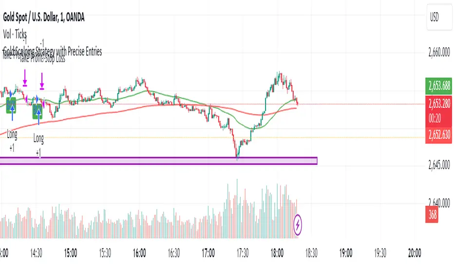
Gold Scalping Strategy with Precise EntriesThe Gold Scalping Strategy with Precise Entries is designed to take advantage of short-term price movements in the gold market (XAU/USD). This strategy uses a combination of technical indicators and chart patterns to identify precise buy and sell opportunities during times of consolidation and trend continuation.
Key Elements of the Strategy:
Exponential Moving Averages (EMAs):
50 EMA: Used as the shorter-term moving average to detect the recent price trend.
200 EMA: Used as the longer-term moving average to determine the overall market trend.
Trend Identification:
A bullish trend is identified when the 50 EMA is above the 200 EMA.
A bearish trend is identified when the 50 EMA is below the 200 EMA.
Average True Range (ATR):
ATR (14) is used to calculate the market's volatility and to set a dynamic stop loss based on recent price movements. Higher ATR values indicate higher volatility.
ATR helps define a suitable stop-loss distance from the entry point.
Relative Strength Index (RSI):
RSI (14) is used as a momentum oscillator to detect overbought or oversold conditions.
However, in this strategy, the RSI is primarily used as a consolidation filter to look for neutral zones (between 45 and 55), which may indicate a potential breakout or trend continuation after a consolidation phase.
Engulfing Patterns:
Bullish Engulfing: A bullish signal is generated when the current candle fully engulfs the previous bearish candle, indicating potential upward momentum.
Bearish Engulfing: A bearish signal is generated when the current candle fully engulfs the previous bullish candle, signaling potential downward momentum.
Precise Entry Conditions:
Long (Buy):
The 50 EMA is above the 200 EMA (bullish trend).
The RSI is between 45 and 55 (neutral/consolidation zone).
A bullish engulfing pattern occurs.
The price closes above the 50 EMA.
Short (Sell):
The 50 EMA is below the 200 EMA (bearish trend).
The RSI is between 45 and 55 (neutral/consolidation zone).
A bearish engulfing pattern occurs.
The price closes below the 50 EMA.
Take Profit and Stop Loss:
Take Profit: A fixed 20-pip target (where 1 pip = 0.10 movement in gold) is used for each trade.
Stop Loss: The stop-loss is dynamically set based on the ATR, ensuring that it adapts to current market volatility.
Visual Signals:
Buy and sell signals are visually plotted on the chart using green and red labels, indicating precise points of entry.
Advantages of This Strategy:
Trend Alignment: The strategy ensures that trades are taken in the direction of the overall trend, as indicated by the 50 and 200 EMAs.
Volatility Adaptation: The use of ATR allows the stop loss to adapt to the current market conditions, reducing the risk of premature exits in volatile markets.
Precise Entries: The combination of engulfing patterns and the neutral RSI zone provides a high-probability entry signal that captures momentum after consolidation.
Quick Scalping: With a fixed 20-pip profit target, the strategy is designed to capture small price movements quickly, which is ideal for scalping.
This strategy can be applied to lower timeframes (such as 1-minute, 5-minute, or 15-minute charts) for frequent trade opportunities in gold trading, making it suitable for day traders or scalpers. However, proper risk management should always be used due to the inherent volatility of gold.
"the strat" için komut dosyalarını ara
Trend Confirmation and ASO-based StrategyStrategy Name: Trend Confirmation with EMA, ASO, and ATR Bands Auto-Trading
Purpose:
This strategy aims to enhance trend confirmation and entry point precision by combining multiple technical indicators. Specifically, it uses the 200 EMA for trend confirmation, the Average Sentiment Oscillator (ASO) to capture market sentiment, and ATR bands for risk management. This provides a comprehensive approach to capturing trade opportunities. The strategy emphasizes trend-following trades, reducing noise while keeping risk management simple.
Uniqueness and Usefulness:
Uniqueness:
This strategy stands out because it integrates multiple elements that complement each other for increased effectiveness and originality. Instead of relying on a single indicator, it generates more accurate trading signals by allowing each indicator to work synergistically.
200 EMA: Used to confirm the long-term trend, providing clarity on the trend direction and ensuring trades align with the dominant market trend.
Average Sentiment Oscillator (ASO): Measures market sentiment based on the crossover between the bull and bear lines. Signals are generated only when ASO detects a trend shift, filtering out price fluctuations and noise.
ATR Bands: Evaluates market volatility and sets stop-loss levels upon entry. By using ATR bands, the strategy supports traders in maintaining a fixed stop-loss for risk management.
Each component analyzes the market from a different perspective, and together, they generate reliable signals for trend-following trades. These indicators are not simply combined but are clearly defined in their roles to improve signal quality.
Usefulness:
This strategy is suitable for medium to long-term traders who focus on trend-following. It emphasizes entry during the early stages of a trend and focuses on risk management by offering reliable signals with minimal noise. The combination of ASO and ATR bands allows traders to assess market volatility while setting take profit levels based on a risk-reward ratio. This helps avoid overreacting to short-term price fluctuations and supports sustainable trading practices.
Entry Conditions:
Long Entry:
Condition: Price is above the 200 EMA, and the ASO bull line crosses above the bear line while also exceeding the 50 level.
Signal: A buy signal is generated, indicating the start of an uptrend.
Short Entry:
Condition: Price is below the 200 EMA, and the ASO bear line crosses above the bull line while also exceeding the 50 level.
Signal: A sell signal is generated, indicating the start of a downtrend.
Exit Conditions:
Exit Strategy:
While this strategy automates both entries and exits, it is recommended that traders manually manage their positions for risk control when necessary. The stop-loss is set based on ATR bands at the time of entry, and a take-profit is set with a risk-reward ratio of 1:1.5.
Risk Management:
This strategy incorporates a fixed stop-loss mechanism, where the stop-loss is set at entry based on the ATR band value. Once set, the stop-loss remains fixed, ensuring that trades stay within a predetermined risk range. The take-profit is based on a risk-reward ratio of 1:1.5, increasing the potential reward relative to the risk.
Account Size: ¥100,000
Commissions and Slippage: Assumed commission of 94 pips per trade and slippage of 1 pip.
Risk per Trade: 10% of account equity (adjustable based on risk tolerance).
Configurable Options:
ASO Period: Period setting for the Average Sentiment Oscillator (default is 32).
ATR Multiplier: Multiplier for ATR band calculation (default is 2.0).
EMA Period: Settings for the 200 EMA.
Signal Display Control: Option to toggle entry signal visibility on or off.
Adequate Sample Size:
To verify the effectiveness of this strategy, it is recommended to conduct extensive backtesting over a long period, covering different market conditions, including both high and low volatility environments.
Credits:
Acknowledgments:
This strategy integrates technical approaches based on the Average Sentiment Oscillator, 200 EMA, and ATR bands, drawing insights from the broader trading community.
Clean Chart Description:
Chart Appearance:
This strategy maintains a clean chart display by offering a toggle to switch the visibility of the ASO, EMA, and entry signals on or off. This helps reduce visual clutter and enhances effective trend analysis.
Addressing the House Rule Violations:
Omissions and Unrealistic Claims:
This strategy makes no exaggerated claims or guarantees about performance. All signals are provided for educational purposes, and it is emphasized that past performance does not guarantee future results. Proper risk management is essential, and the importance of this is highlighted throughout the strategy.
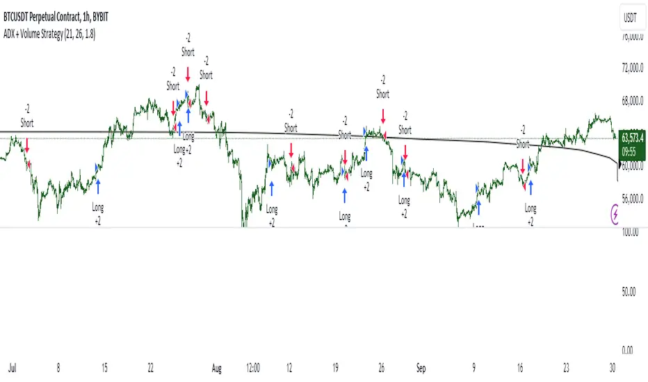
ADX + Volume Strategy### Strategy Description: ADX and Volume-Based Trading Strategy
This strategy is designed to identify strong market trends using the **Average Directional Index (ADX)** and confirm trading signals with **Volume**. The idea behind the strategy is to enter trades only when the market shows a strong trend (as indicated by ADX) and when the price movement is supported by high trading volume. This combination helps filter out weaker signals and provides more reliable entries into positions.
### Key Indicators:
1. **ADX (Average Directional Index)**:
- **Purpose**: ADX is a technical indicator that measures the strength of a trend, regardless of its direction (up or down).
- **Usage**: The strategy uses ADX to determine whether the market is trending strongly. If ADX is above a certain threshold (default is 25), it indicates that a strong trend is present.
- **Directional Indicators**:
- **DI+ (Directional Indicator Plus)**: Indicates the strength of the upward price movement.
- **DI- (Directional Indicator Minus)**: Indicates the strength of the downward price movement.
- ADX does not indicate the direction of the trend but confirms that a trend exists. DI+ and DI- are used to determine the direction.
2. **Volume**:
- **Purpose**: Volume is a key indicator for confirming the strength of a price movement. High volume suggests that a large number of market participants are supporting the movement, making it more likely to continue.
- **Usage**: The strategy compares the current volume to the 20-period moving average of the volume. The trade signal is confirmed if the current volume is greater than the average volume by a specified **Volume Multiplier** (default multiplier is 1.5). This ensures that the trade is supported by strong market participation.
### Strategy Logic:
#### **Entry Conditions:**
1. **Long Position** (Buy):
- **ADX** is above the threshold (default is 25), indicating a strong trend.
- **DI+ > DI-**, signaling that the market is trending upward.
- The **current volume** is greater than the 20-period average volume multiplied by the **Volume Multiplier** (e.g., 1.5), indicating that the upward price movement is backed by sufficient market activity.
2. **Short Position** (Sell):
- **ADX** is above the threshold (default is 25), indicating a strong trend.
- **DI- > DI+**, signaling that the market is trending downward.
- The **current volume** is greater than the 20-period average volume multiplied by the **Volume Multiplier** (e.g., 1.5), indicating that the downward price movement is backed by strong selling activity.
#### **Exit Conditions**:
- Positions are closed when the opposite signal appears:
- **For long positions**: Close when the short conditions are met (ADX still above the threshold, DI- > DI+, and the volume condition holds).
- **For short positions**: Close when the long conditions are met (ADX still above the threshold, DI+ > DI-, and the volume condition holds).
### Parameters:
- **ADX Period**: The period used to calculate ADX (default is 14). This controls how sensitive the ADX is to price movements.
- **ADX Threshold**: The minimum ADX value required for the strategy to consider the market trend as strong (default is 25). Higher values focus on stronger trends.
- **Volume Multiplier**: This parameter adjusts how much higher the current volume needs to be compared to the 20-period moving average for the signal to be valid. A value of 1.5 means the current volume must be 50% higher than the average volume.
### Example Trade Flow:
1. **Long Trade Example**:
- ADX > 25, confirming a strong trend.
- DI+ > DI-, confirming that the trend direction is upward.
- The current volume is 50% higher than the 20-period average volume (multiplied by 1.5).
- **Action**: Enter a long position.
2. **Short Trade Example**:
- ADX > 25, confirming a strong trend.
- DI- > DI+, confirming that the trend direction is downward.
- The current volume is 50% higher than the 20-period average volume.
- **Action**: Enter a short position.
### Strengths of the Strategy:
- **Trend Filtering**: The strategy ensures that trades are only taken when the market is trending strongly (confirmed by ADX) and that the price movement is supported by high volume, reducing the likelihood of false signals.
- **Volume Confirmation**: Using volume as confirmation provides an additional layer of reliability, as volume spikes often accompany sustained price moves.
- **Dual Signal Confirmation**: Both trend strength (ADX) and volume conditions must be met for a trade, making the strategy more robust.
### Weaknesses of the Strategy:
- **Limited Effectiveness in Range-Bound Markets**: Since the strategy relies on strong trends, it may underperform in sideways or non-trending markets where ADX stays below the threshold.
- **Lagging Nature of ADX**: ADX is a lagging indicator, which means that it may confirm the trend after it has already begun, potentially leading to late entries.
- **Volume Requirement**: In low-volume markets, the volume multiplier condition may not be met often, leading to fewer trade opportunities.
### Customization:
- **Adjust the ADX Threshold**: You can raise the threshold if you want to focus only on very strong trends, or lower it to capture moderate trends.
- **Adjust the Volume Multiplier**: You can change the multiplier to be more or less strict. A higher multiplier (e.g., 2.0) will require a stronger volume spike to confirm the signal, while a lower multiplier (e.g., 1.2) will allow more trades with weaker volume confirmation.
### Summary:
This ADX and Volume strategy is ideal for traders who want to follow strong trends while ensuring that the trend is supported by high trading volume. By combining a trend strength filter (ADX) and volume confirmation, the strategy aims to increase the probability of entering profitable trades while reducing the number of false signals. However, it may underperform in range-bound markets or in markets with low volume.
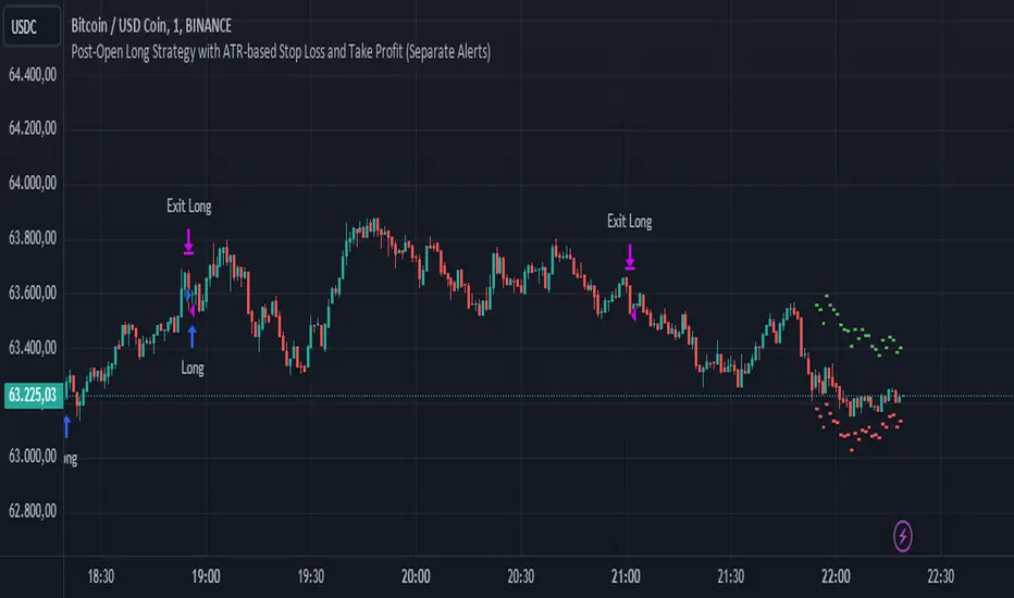
Post-Open Long Strategy with ATR-based Stop Loss and Take ProfitThe "Post-Open Long Strategy with ATR-Based Stop Loss and Take Profit" is designed to identify buying opportunities after the German and US markets open. It combines various technical indicators to filter entry signals, focusing on breakout moments following price lateralization periods.
Key Components and Their Interaction:
Bollinger Bands (BB):
Description: Uses BB with a 14-period length and standard deviation multiplier of 1.5, creating narrower bands for lower timeframes.
Role in the Strategy: Identifies low volatility phases (lateralization). The lateralization condition is met when the price is near the simple moving average of the BB, suggesting an imminent increase in volatility.
Exponential Moving Averages (EMA):
10-period EMA: Quickly detects short-term trend direction.
200-period EMA: Filters long-term trends, ensuring entries occur in a bullish market.
Interaction: Positions are entered only if the price is above both EMAs, indicating a consolidated positive trend.
Relative Strength Index (RSI):
Description: 7-period RSI with a threshold above 30.
Role in the Strategy: Confirms the market is not oversold, supporting the validity of the buy signal.
Average Directional Index (ADX):
Description: 7-period ADX with 7-period smoothing and a threshold above 10.
Role in the Strategy: Assesses trend strength. An ADX above 10 indicates sufficient momentum to justify entry.
Average True Range (ATR) for Dynamic Stop Loss and Take Profit:
Description: 14-period ATR with multipliers of 2.0 for Stop Loss and 4.0 for Take Profit.
Role in the Strategy: Adjusts exit levels based on current volatility, enhancing risk management.
Resistance Identification and Breakout:
Description: Analyzes the highs of the last 20 candles to identify resistance levels with at least two touches.
Role in the Strategy: A breakout above this level signals a potential continuation of the bullish trend.
Time Filters and Market Conditions:
Trading Hours: Operates only during the opening of the German market (8:00 - 12:00) and US market (15:30 - 19:00).
Panic Candle: The current candle must close negative, leveraging potential emotional reactions in the market.
Avoiding Entry During Pullbacks:
Description: Checks that the two previous candles are not both bearish.
Role in the Strategy: Avoids entering during a potential pullback, improving trade success probability.
Post-Open Long Strategy with ATR-Based Stop Loss and Take Profit
The "Post-Open Long Strategy with ATR-Based Stop Loss and Take Profit" is designed to identify buying opportunities after the German and US markets open. It combines various technical indicators to filter entry signals, focusing on breakout moments following price lateralization periods.
Key Components and Their Interaction:
Bollinger Bands (BB):
Description: Uses BB with a 14-period length and standard deviation multiplier of 1.5, creating narrower bands for lower timeframes.
Role in the Strategy: Identifies low volatility phases (lateralization). The lateralization condition is met when the price is near the simple moving average of the BB, suggesting an imminent increase in volatility.
Exponential Moving Averages (EMA):
10-period EMA: Quickly detects short-term trend direction.
200-period EMA: Filters long-term trends, ensuring entries occur in a bullish market.
Interaction: Positions are entered only if the price is above both EMAs, indicating a consolidated positive trend.
Relative Strength Index (RSI):
Description: 7-period RSI with a threshold above 30.
Role in the Strategy: Confirms the market is not oversold, supporting the validity of the buy signal.
Average Directional Index (ADX):
Description: 7-period ADX with 7-period smoothing and a threshold above 10.
Role in the Strategy: Assesses trend strength. An ADX above 10 indicates sufficient momentum to justify entry.
Average True Range (ATR) for Dynamic Stop Loss and Take Profit:
Description: 14-period ATR with multipliers of 2.0 for Stop Loss and 4.0 for Take Profit.
Role in the Strategy: Adjusts exit levels based on current volatility, enhancing risk management.
Resistance Identification and Breakout:
Description: Analyzes the highs of the last 20 candles to identify resistance levels with at least two touches.
Role in the Strategy: A breakout above this level signals a potential continuation of the bullish trend.
Time Filters and Market Conditions:
Trading Hours: Operates only during the opening of the German market (8:00 - 12:00) and US market (15:30 - 19:00).
Panic Candle: The current candle must close negative, leveraging potential emotional reactions in the market.
Avoiding Entry During Pullbacks:
Description: Checks that the two previous candles are not both bearish.
Role in the Strategy: Avoids entering during a potential pullback, improving trade success probability.
Entry and Exit Conditions:
Long Entry:
The price breaks above the identified resistance.
The market is in a lateralization phase with low volatility.
The price is above the 10 and 200-period EMAs.
RSI is above 30, and ADX is above 10.
No short-term downtrend is detected.
The last two candles are not both bearish.
The current candle is a "panic candle" (negative close).
Order Execution: The order is executed at the close of the candle that meets all conditions.
Exit from Position:
Dynamic Stop Loss: Set at 2 times the ATR below the entry price.
Dynamic Take Profit: Set at 4 times the ATR above the entry price.
The position is automatically closed upon reaching the Stop Loss or Take Profit.
How to Use the Strategy:
Application on Volatile Instruments:
Ideal for financial instruments that show significant volatility during the target market opening hours, such as indices or major forex pairs.
Recommended Timeframes:
Intraday timeframes, such as 5 or 15 minutes, to capture significant post-open moves.
Parameter Customization:
The default parameters are optimized but can be adjusted based on individual preferences and the instrument analyzed.
Backtesting and Optimization:
Backtesting is recommended to evaluate performance and make adjustments if necessary.
Risk Management:
Ensure position sizing respects risk management rules, avoiding risking more than 1-2% of capital per trade.
Originality and Benefits of the Strategy:
Unique Combination of Indicators: Integrates various technical metrics to filter signals, reducing false positives.
Volatility Adaptability: The use of ATR for Stop Loss and Take Profit allows the strategy to adapt to real-time market conditions.
Focus on Post-Lateralization Breakout: Aims to capitalize on significant moves following consolidation periods, often associated with strong directional trends.
Important Notes:
Commissions and Slippage: Include commissions and slippage in settings for more realistic simulations.
Capital Size: Use a realistic trading capital for the average user.
Number of Trades: Ensure backtesting covers a sufficient number of trades to validate the strategy (ideally more than 100 trades).
Warning: Past results do not guarantee future performance. The strategy should be used as part of a comprehensive trading approach.
With this strategy, traders can identify and exploit specific market opportunities supported by a robust set of technical indicators and filters, potentially enhancing their trading decisions during key times of the day.
Trend Magic with EMA, SMA, and Auto-TradingRelease Notes
Strategy Name: Trend Magic with EMA, SMA, and Auto-Trading
Purpose: This strategy is designed to capture entry and exit points in the market using the Trend Magic indicator and three moving averages (EMA45, SMA90, and SMA180). Specifically, it uses the perfect order of the moving averages and the color changes in Trend Magic to identify trend reversals and potential trading opportunities.
Uniqueness and Usefulness
Uniqueness: The strategy utilizes the Trend Magic indicator, which is based on price and volatility, along with three moving averages to assess the strength of trends. The signals are generated only when the moving averages are in perfect order, and the Trend Magic color changes, ensuring that the entry is made during established trends. This combination provides a higher degree of reliability compared to strategies that rely solely on price action or single indicators.
Usefulness: This strategy is particularly useful for traders looking to capture trends over longer periods. It is effective at reducing noise in the market, only providing signals when the moving averages align and the Trend Magic indicator confirms a trend reversal. It works well in both trending and volatile markets.
Entry Conditions
Long Entry:
Condition: A perfect order (EMA45 > SMA90 > SMA180) is established, and Trend Magic changes color from red to blue.
Signal: A buy signal is generated, indicating the start of an uptrend.
Short Entry:
Condition: A perfect order (EMA45 < SMA90 < SMA180) is established, and Trend Magic changes color from blue to red.
Signal: A sell signal is generated, indicating the start of a downtrend.
Exit Conditions
Exit Strategy:
This strategy automatically enters and exits trades based on signals, but traders are encouraged to manage exits manually according to their own risk management preferences. The strategy includes stop loss and take profit settings based on risk-to-reward ratios for better risk management.
Risk Management
The strategy includes built-in risk management by using the SMA90 level at the time of entry as the stop-loss point and setting the take profit at a 1:1.5 risk-to-reward ratio. The stop-loss level is fixed at the entry point and does not move as the market progresses. Traders are advised to implement additional risk management, such as trailing stops, for added protection.
Account Size: ¥100,000
Commissions and Slippage: Assumes 94 pips for commissions and 1 pip for slippage per trade
Risk per Trade: 10% of account equity (adjust this based on personal risk tolerance)
Configurable Options
Configurable Options:
CCI Period: Set the period for the CCI used to calculate the Trend Magic indicator (default is 21).
ATR Multiplier: Set the multiplier for ATR used in the Trend Magic calculation (default is 1.0).
EMA/SMA Periods: The periods for the three moving averages (default is EMA45, SMA90, and SMA180).
Signal Display Control: An option to toggle the display of buy and sell signals on the chart.
Adequate Sample Size
To ensure the robustness and reliability of this strategy, it is recommended to backtest it with a sufficiently long period of historical data. Testing across different market conditions, including high and low volatility periods, is also advised.
Credits
Acknowledgments:
This strategy is based on the Trend Magic indicator combined with moving averages and draws on contributions from the technical analysis and trading community.
Clean Chart Description
Chart Appearance:
To maintain a clean and simple chart, this strategy includes options to turn off the display of Trend Magic, moving averages, and entry signals. Traders can adjust these display settings as needed to minimize visual clutter and focus on effective trend analysis.
Addressing the House Rule Violations
Omissions and Unrealistic Claims
Clarification:
This strategy does not make any unrealistic or unsupported claims about its performance. All signals are intended for educational purposes only and do not guarantee future results. It is important to note that past performance does not guarantee future outcomes, and proper risk management is crucial.

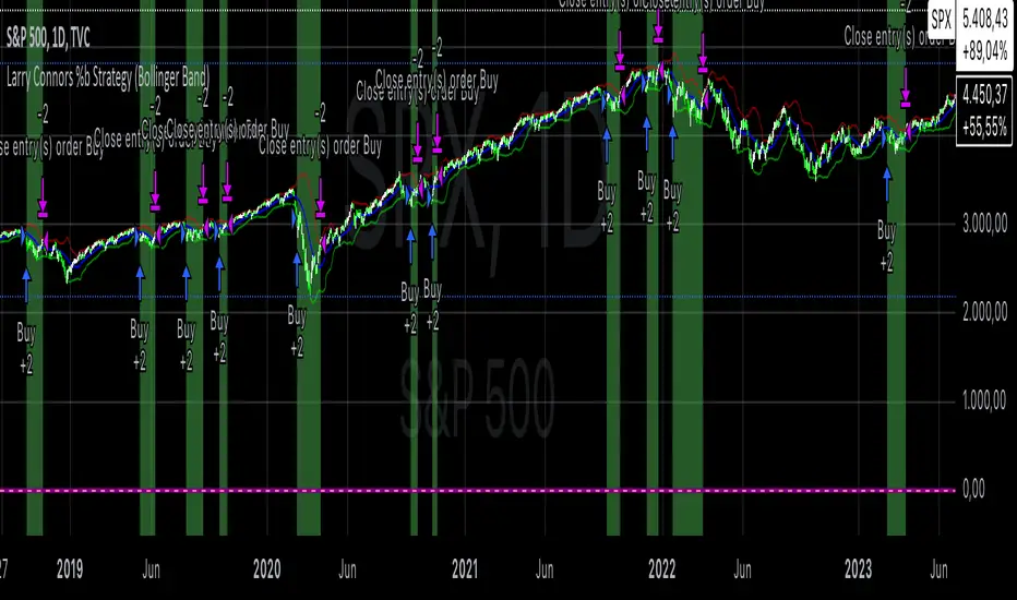
Larry Connors %b Strategy (Bollinger Band)Larry Connors’ %b Strategy is a mean-reversion trading approach that uses Bollinger Bands to identify buy and sell signals based on the %b indicator. This strategy was developed by Larry Connors, a renowned trader and author known for his systematic, data-driven trading methods, particularly those focusing on short-term mean reversion.
The %b indicator measures the position of the current price relative to the Bollinger Bands, which are volatility bands placed above and below a moving average. The strategy specifically targets times when prices are oversold within a long-term uptrend and aims to capture rebounds by buying at relatively low points and selling at relatively high points.
Strategy Rules
The basic rules of the %b Strategy are:
1. Trend Confirmation: The closing price must be above the 200-day moving average. This filter ensures that trades are made in alignment with a longer-term uptrend, thereby avoiding trades against the primary market trend.
2. Oversold Conditions: The %b indicator must be below 0.2 for three consecutive days. The %b value below 0.2 indicates that the price is near the lower Bollinger Band, suggesting an oversold condition.
3. Entry Signal: Enter a long position at the close when conditions 1 and 2 are met.
4. Exit Signal: Exit the position when the %b value closes above 0.8, signaling an overbought condition where the price is near the upper Bollinger Band.
How the Strategy Works
This strategy operates on the premise of mean reversion, which suggests that extreme price movements will revert to the mean over time. By entering positions when the %b value indicates an oversold condition (below 0.2) in a confirmed uptrend, the strategy attempts to capture short-term price rebounds. The exit rule (when %b is above 0.8) aims to lock in profits once the price reaches an overbought condition, often near the upper Bollinger Band.
Who Was Larry Connors?
Larry Connors is a well-known figure in the world of financial markets and trading. He co-authored several influential trading books, including “Short-Term Trading Strategies That Work” and “High Probability ETF Trading.” Connors is recognized for his quantitative approach, focusing on systematic, rules-based strategies that leverage historical data to validate trading edges.
His work primarily revolves around short-term trading strategies, often using technical indicators like RSI (Relative Strength Index), Bollinger Bands, and moving averages. Connors’ methodologies have been widely adopted by traders seeking structured approaches to exploit short-term inefficiencies in the market.
Risks of the Strategy
While the %b Strategy can be effective, particularly in mean-reverting markets, it is not without risks:
1. Mean Reversion Assumption: The strategy is based on the assumption that prices will revert to the mean. In trending or sharply falling markets, this reversion may not occur, leading to sustained losses.
2. False Signals in Choppy Markets: In volatile or sideways markets, the strategy may generate multiple false signals, resulting in whipsaw trades that can erode capital through frequent small losses.
3. No Stop Loss: The basic implementation of the strategy does not include a stop loss, which increases the risk of holding losing trades longer than intended, especially if the market continues to move against the position.
4. Performance During Market Crashes: During major market downturns, the strategy’s buy signals could be triggered frequently as prices decline, compounding losses without the presence of a risk management mechanism.
Scientific References and Theoretical Basis
The %b Strategy relies on the concept of mean reversion, which has been extensively studied in finance literature. Studies by Avellaneda and Lee (2010) and Bouchaud et al. (2018) have demonstrated that mean-reverting strategies can be profitable in specific market environments, particularly when combined with volatility filters like Bollinger Bands. However, the same studies caution that such strategies are highly sensitive to market conditions and often perform poorly during periods of prolonged trends.
Bollinger Bands themselves were popularized by John Bollinger and are widely used to assess price volatility and detect potential overbought and oversold conditions. The %b value is a critical part of this analysis, as it standardizes the position of price relative to the bands, making it easier to compare conditions across different securities and time frames.
Conclusion
Larry Connors’ %b Strategy is a well-known mean-reversion technique that leverages Bollinger Bands to identify buying opportunities in uptrending markets when prices are temporarily oversold. While the strategy can be effective under the right conditions, traders should be aware of its limitations and risks, particularly in trending or highly volatile markets. Incorporating risk management techniques, such as stop losses, could help mitigate some of these risks, making the strategy more robust against adverse market conditions.
TRIN (Arms Index) Trading StrategyThe TRIN (Arms Index), also known as the Short-Term Trading Index, is a technical indicator designed to gauge the internal strength or weakness of the market. It compares the number of advancing and declining stocks to the advancing and declining volume (AD Volume). A TRIN value above 1.0 generally indicates bearish market conditions, while a value below 1.0 suggests bullish market sentiment.
Strategy Rules:
Entry Condition (Long Position): When the TRIN value is above 1.0, the strategy enters a long position, indicating that the market may be oversold, and a potential reversal could occur.
Exit Condition: The strategy exits the long position when the closing price is higher than the previous day’s high, signaling a potential rebound in the market.
This strategy aims to capitalize on short-term market inefficiencies by entering trades during periods of potential market weakness and exiting when signs of recovery appear.
How the TRIN Index Works:
The TRIN is calculated as follows:
TRIN=Advancing Issues / Declining IssuesAdvancing Volume / Declining Volume
TRIN=Advancing Volume / Declining VolumeAdvancing Issues / Declining Issues
A TRIN value above 1.0 indicates that the market is potentially oversold (more declining stocks with higher volume), while a value below 1.0 suggests the market may be overbought (more advancing stocks with higher volume) .
Empirical Evidence:
Market Sentiment Indicator: The TRIN has been widely used as a sentiment indicator. Research by Zweig (1997) suggests that extreme TRIN values can serve as a contrarian signal, indicating potential turning points in the market. For instance, a TRIN above 2.0 is often considered a sign of panic selling, which can precede a market bottom .
Overbought/Oversold Conditions: Studies have shown that indicators like TRIN, which measure market breadth and volume, can be effective in identifying overbought and oversold conditions. According to Fama and French (1988), market sentiment indicators that consider both price and volume data can offer insights into future price movements .
Risks and Limitations:
False Signals:
One of the primary risks of using the TRIN-based strategy is the possibility of false signals. A TRIN value above 1.0 does not always guarantee a market rebound, especially in sustained bearish trends. In such cases, the strategy might enter long positions prematurely, leading to losses.
Research by Brock, Lakonishok, and LeBaron (1992) found that while market indicators like TRIN can be useful, they are not foolproof and can generate multiple false positives, particularly in volatile markets .
Market Regimes:
The effectiveness of the TRIN index can vary depending on the market regime. In strongly trending markets, either bullish or bearish, the TRIN may not provide reliable reversal signals, and relying on it could result in trades that go against the prevailing trend. For instance, during strong bear markets, the TRIN may frequently remain above 1.0, leading to multiple losing trades as the market continues to decline.
Short-Term Focus:
The TRIN strategy is inherently short-term focused, aiming to capture quick market reversals. This makes it sensitive to market noise and less effective for longer-term investors. Moreover, short-term trading strategies often require more frequent adjustments and can incur higher transaction costs, which may erode profitability over time.
Liquidity and Execution Risk:
Since the TRIN strategy requires entering and exiting trades based on short-term market movements, it is vulnerable to liquidity and execution risks. In fast-moving markets, the execution of trades may be delayed, leading to slippage and potentially unfavorable entry or exit points.
Conclusion:
The TRIN (Arms Index) Trading Strategy can be an effective tool for traders looking to capitalize on short-term market inefficiencies and potential reversals. However, it is important to recognize the risks associated with this strategy, including false signals, sensitivity to market regimes, and execution risks. Traders should employ proper risk management techniques and consider combining the TRIN with other indicators to improve the robustness of the strategy.
While the TRIN provides valuable insights into market sentiment, it is not a standalone solution and should be used in conjunction with a broader trading plan that takes into account both technical and fundamental analysis.
References:
Arms, Richard W. "Volume Adjusted Moving Averages." Technical Analysis of Stocks & Commodities, 1993.
Zweig, Martin. Winning on Wall Street. Warner Books, 1997.
Fama, Eugene F., and Kenneth R. French. "Permanent and Temporary Components of Stock Prices." Journal of Political Economy, 1988.
Brock, William, Josef Lakonishok, and Blake LeBaron. "Simple Technical Trading Rules and the Stochastic Properties of Stock Returns." Journal of Finance, 1992.

Averaging Down Strategy1. Averaging Down:
Definition: "Averaging Down" is a strategy in which an investor buys more shares of a declining asset, thus lowering the average purchase price. The main idea is that, by averaging down, the investor can recover faster when the price eventually rebounds.
Risk Considerations: This strategy assumes that the asset will recover in value. If the price continues to decline, however, the investor may suffer larger losses. Academic research highlights the psychological bias of loss aversion that often leads investors to engage in averaging down, despite the increased risk (Barberis & Huang, 2001).
2. RSI (Relative Strength Index):
Definition: The RSI is a momentum oscillator that measures the speed and change of price movements. It ranges from 0 to 100 and is commonly used to identify overbought or oversold conditions. A reading below 30 (or in this case, 35) typically indicates an oversold condition, which might suggest a potential buying opportunity (Wilder, 1978).
Risk Considerations: RSI-based strategies can produce many false signals in range-bound or choppy markets, where prices do not exhibit strong trends. This can lead to multiple losing trades and an overall negative performance (Gencay, 1998).
3. Combination of RSI and Price Movement:
Approach: The combination of RSI for entry signals and price movement (previous day's high) for exit signals aims to capture short-term market reversals. This hybrid approach attempts to balance momentum with price confirmation.
Risk Considerations: While this combination can work well in trending markets, it may struggle in volatile or sideways markets. Additionally, a significant risk of averaging down is that the trader may continue adding to a losing position, which can exacerbate losses if the price keeps falling.
Risk Warnings:
Increased Losses Through Averaging Down:
Averaging down involves buying more of a falling asset, which can increase exposure to downside risk. Studies have shown that this approach can lead to larger losses when markets continue to decline, especially during prolonged bear markets (Statman, 2004).
A key risk is that this strategy may lead to significant capital drawdowns if the price of the asset does not recover as expected. In the worst-case scenario, this can result in a total loss of the invested capital.
False Signals with RSI:
RSI-based strategies are prone to generating false signals, particularly in markets that do not exhibit strong trends. For example, Gencay (1998) found that while RSI can be effective in certain conditions, it often fails in choppy or range-bound markets, leading to frequent stop-outs and drawdowns.
Psychological Bias:
Behavioral finance research suggests that the "Averaging Down" strategy may be influenced by loss aversion, a bias where investors prefer to avoid losses rather than achieve gains (Kahneman & Tversky, 1979). This can lead to poor decision-making, as investors continue to add to losing positions in the hope of a recovery.
Empirical Studies:
Gencay (1998): The study "The Predictability of Security Returns with Simple Technical Trading Rules" found that technical indicators like RSI can provide predictive value in certain markets, particularly in volatile environments. However, they are less reliable in markets that lack clear trends.
Barberis & Huang (2001): Their research on behavioral biases, including loss aversion, explains why investors are often tempted to average down despite the risks, as they attempt to avoid realizing losses.
Statman (2004): In "The Diversification Puzzle," Statman discusses how strategies like averaging down can increase risk exposure without necessarily improving long-term returns, especially if the underlying asset continues to perform poorly.
Conclusion:
The "Averaging Down Strategy with RSI" combines elements of technical analysis with a psychologically-driven averaging down approach. While the strategy may offer opportunities in trending or oversold markets, it carries significant risks, particularly in volatile or declining markets. Traders should be cautious when using this strategy, ensuring they manage risk effectively and avoid overexposure to a losing position.

Dow Theory based Strategy (Markttechnik)What makes this script unique?
calculates two trends at the same time: a big one for the overall strong trend - and a small one to trigger a trade after a small correction within the big trend
only if both trends (the small and the big trend) are in an uptrend, a buy signal is created: this prevents a buy signal from being generated in a falling market just because an upward movement begins in a small trend
the exit strategy can be configured very flexibly and individually: use the last low as stop loss and automatically switch to a trialing stop loss as soon as the take profit is reached (instead of finishing the trade)
the take profit strategy can also be configured - e.g. use the last high, a fixed percentage or a combination of it
plots each trade in detail on the chart - e.g. inner candles or the exact progression of the stop loss over the entire duration of the trade to allow you to analyze each trade precisely
What does the script do and how?
In this strategy an intact upward trend is characterized by higher highs and lower lows only if the big trend and the small trend are in an upward trend at the same time.
The following describes how the script calculates a buy signal. Every step is drawn to the chart immediately - see example chart above:
1. the stock rises in the big trend - i.e. in a longer time frame
2. a correction takes place (the share price falls) - but does not create a new low
3. the stock rises again in the big trend and creates a new high
From now on, the big trend is in an intact upward trend (until it falls below its last low).
This is drawn to the chart as 3 bold green zigzag lines.
But we do not buy right now! Instead, we want to wait for a correction in the big trend and for the start of a small upward trend.
4. a correction takes place (not below the low from 2.)
Now, the script also starts to calculate the small trend:
5. the stock rises in the small trend - i.e. in a shorter time frame
6. a small correction takes place (not below the low from 4.)
7. the stock rises above the high from 5.: a new high in the shorter time frame
Now, both trends are in an intact upward trend.
A buy signal is created and both the minor and major trend are colored green on the chart.
Now, the trade is active and:
the stop loss is calculated and drawn for each candle
the take profit is calculated and drawn to the chart
as soon as the price reaches the take profit or the stop loss, the trade is closed
Features and functionalities
Uptrend : An intact upward trend is characterized by higher highs and lower lows. Uptrends are shown in green on the chart.
The beginning of an uptrend is numbered 1, each subsequent high is numbered 2, and each low is numbered 3.
Downtrend: An intact downtrend is characterized by lower highs and lower lows. Downtrends are displayed in red on the chart.
Note that our indicator does not show the numbering of the points of the downtrend.
Trendless phases: If there is no intact trend, we are in a trendless phase. Trendless phases are shown in blue on the chart.
This occurs after an uptrend, when a lower low or a lower high is formed. Or after a downtrend, when a higher low or a higher high is formed.
Buy signals
A buy signal is generated as soon as a new upward trend has been formed or a new high has been established in an intact upward trend.
But even before a buy signal is generated, this strategy anticipates a possible emerging trend and draws the next possible trading opportunity to the chart.
In addition to the (not yet reached) buy price, the risk-reward ratio, the StopLoss and the TakeProfit price is shown.
With this information, you can already enter a StopBuy order, which is thus triggered directly with the then created buy signal.
You can configure, if a buy signal shall be created while the big trend is an uptrend, a downtrend and/or trendless.
Exit strategy
With this strategy, you have multiple possibilities to close your position. All of them can be configured within the settings. In general, you can combine a take profit strategy with a stop loss strategy.
The take profit price will be calculated once for each trade. It will be drawn to the chart for active trade.
Depending on your configuration, this can be the last high (which is often a resistance level), a fixed percentage added to the buy price or the maximum of both.
You can also configure that a trailing stop loss is used as soon as the take profit price is reached once.
The stop loss gets recalculated with each candle and is displayed and plotted for each active and finished trade. With this, you can easily check how the stop loss changed during your trades.
The stop loss can be configured flexibly:
Use the classic "trailing stop loss" that follows the price from below.
Set the stop loss to the last low and tighten it every time the small trend marks a new local low.
Confiure that the stop loss is tightened as soon as the break even is reached. Nothing is more annoying than a trade turning from a win to a loss.
Ignore inside candles (see description below) and relax the stop loss to use the outside candle for its calculation.
Inner candles
Inner candles are created when the candle body is within the maximum values of a previous candle (the outer candle). There can be any number of consecutive inner candles. As soon as you have activated the "Check inner candles" setting, all consecutive inner candles will be highlighted in yellow on the chart.
Prices during an inner candle scenario might be irrelevant for trading and can be interpreted as fluctuations within the outside candle. For this reason, the trailing stop loss should not be aligned with inner candles. Therefore, as soon as an inner candle occurs, the stop loss is reset and the low at the time of the outside candle is used as the calculation for the trailing stop loss. This will all be plotted for you on the chart.
Display of the trades:
All active and closed trades of the last 5 years are displayed in the chart with buy signal, sell, stop loss history, inside candles and statistics.
Backtesting:
The strategy can be simulated for each stock over the period of the last 5 years. Each individual trade is recorded and can be traced and analyzed in the chart including stop loss history. Detailed evaluations and statistics are available to evaluate the performance of the strategy.
Additional Statistics
This strategy immediately displays a statistic table to the chart area giving you an overview of its performance over the last years for the given chart.
This includes:
The total win/loss in $ and %
The win/loss per year in %
The active investment time in days and % (e.g. invested 10 of 100 trading days -> 10%)
The total win/loss in %, extrapolated to 100% equity usage: Only with this value can strategies really be compared. Because you are not invested between the trades and could invest in other stocks during this time. This value indicates how much profit you would have made if you had been invested 100% of the time - or to put it another way - if you had been invested 100% of the time in stocks with exactly the same performance. Let's say you had only one trade in the last 5 years that lasted, say, only one month and made 5% profit. This would be significantly better than a strategy with which you were invested for, say, 5 years and made 10% profit.
The total profit/loss per year in %, extrapolated to 100% equity usage
Notifications (alerts):
Get alerted before a new buy signal emerges to create an order if necessary and not miss a trade. You can also be notified when the stop loss needs to be adjusted. The notification can be done in different ways, e.g. by Mail, PopUp or App-Notification. This saves them the annoying, time-consuming and error-prone "click through" all the charts.
Settings: Display Settings
With these settings, you have the possibility to:
Show the small or the big trend as a background color
Configure if the numbers (1-2-3-2-3) shall be shown at all or only for the small, the big trend or both
Settings: Trend calculation - fine tuning
Drawing trend lines on a chart is not an exact science. Some highs and lows are not very clear or significant. And so it will always happen that 2 different people would draw different trendlines for the same chart. Unfortunately, there is no exact "right" or "wrong" here.
With the options under "Trend Calculation - Fine Tuning" you have the possibility to influence the drawing in of trends and to adapt it to your personal taste.
Small Trend, Big Trend : With these settings you can influence how significant a high or low has to be to recognize them as an independent high or low. The larger the values, the more significant a high or low must be to be recognized as such.
High and low recognition : With this setting you can influence when two adjacent, almost identical highs or lows should be recognized as independent highs or lows. The higher the value, the more different "similar" highs or lows must be in order to be recognized as such.
Which default settings were selected and why
Show Trades: true - its often useful to see all recent trades in the chart
Time Frame: 1 day - most common time frame (except for day traders)
Take Profit: combined 10% - the last high is taken as take profit because the trend often changes there, but only if there is at least 10% profit to ensure we do not risk money for a tiny profit
Stop Loss: combined - the last low is used as stop loss because the trend would break there and switch to a trailing stop loss as soon as our take profit is reached to let our profits run without risking them anymore
Stop Loss distance: 3% - we are giving the price 3% air (below the last low) to avoid being stopped out due to a short price drop
Trailing Stop Loss: 2% - we have to give the stop loss some room to avoid being stopped out prematurely; this is a value that is well balanced between a certain downside distance and the profit-taking ratio
Set Stop Loss to break even: true, 2% - once we reached the break even, it is a common practice to not risk our money anymore, the value is set to the same value as the trailing stop loss
Trade Filter: Uptrend - we only start trades if the big trend is an uptrend in the expectation that it will continue after a small correction
Display settings: those will not influence the trades, feel free to change them to your needs
Trend calculation - Fine Tuning: 1/1,5/0,05; influences the internal calculation for highs and lows and how significant they need to be to be considered a new high or low; the default values will provide you nicely calculated trends in the daily time frame; if there are too many or too few lows and highs according to your taste, feel free to play around and immediately see the result drawn to the chart; read the manual for a detailed description of this values
Note that you can (and should) configure the general trading properties like your initial capital, order size, slippage and commission.

Trend Signals with TP & SL [UAlgo] StrategyThe "Trend Signals with TP & SL Strategy" is a trading strategy designed to capture trend continuation signals while incorporating sophisticated risk management techniques. This strategy is tailored for traders who wish to capitalize on trending market conditions with precise entry and exit points, automatically calculating Take Profit (TP) and Stop Loss (SL) levels based on either Average True Range (ATR) or percentage values. The strategy aims to enhance trade management by preventing multiple simultaneous positions and dynamically adapting to changing market conditions.
This strategy is highly configurable, allowing traders to adjust sensitivity, the ATR calculation method, and the cloud moving average length. Additionally, the strategy can display buy and sell signals directly on the chart, along with visual representation of entry points, stop losses, and take profits. It also features a cloud-based trend analysis using a MACD-driven color fill that indicates the strength and direction of the trend.
🔶 Key Features
Configurable Trend Continuation Signals:
Source Selection: The strategy uses the midpoint of the high-low range as the default source, but it is adjustable.
Sensitivity: The sensitivity of the trend signals can be adjusted using a multiplier, ranging from 0.5 to 5.
ATR Calculation: The strategy allows users to choose between two ATR calculation methods for better adaptability to different market conditions.
Cloud Moving Average: Traders can adjust the cloud moving average length, which is used in conjunction with MACD to provide a visual trend indication.
Take Profit & Stop Loss Management:
ATR-Based or Percent-Based: The strategy offers flexibility in setting TP and SL levels, allowing traders to choose between ATR-based multipliers or fixed percentage values.
Dynamic Adjustment: TP and SL levels are dynamically adjusted according to the selected method, ensuring trades are managed based on real-time market conditions.
Prevention of Multiple Positions:
Single Position Control: To reduce risk and enhance strategy reliability, the strategy includes an option to prevent multiple positions from being opened simultaneously.
Visual Trade Indicators:
Buy/Sell Signals: Clearly displays buy and sell signals on the chart for easy interpretation.
Entry, SL, and TP Lines: Draws lines for entry price, stop loss, and take profit directly on the chart, helping traders to monitor trades visually.
Trend Cloud: A color-filled cloud based on MACD and the cloud moving average provides a visual cue of the trend’s direction and strength.
Performance Summary Table:
In-Chart Statistics: A table in the top right of the chart displays key performance metrics, including total trades, wins, losses, and win rate percentage, offering a quick overview of the strategy’s effectiveness.
🔶 Interpreting the Indicator
Trend Signals: The strategy identifies trend continuation signals based on price action relative to an ATR-based threshold. A buy signal is generated when the price crosses above a key level, indicating an uptrend. Conversely, a sell signal occurs when the price crosses below a level, signaling a downtrend.
Cloud Visualization: The cloud, derived from MACD and moving averages, changes color to reflect the current trend. A positive cloud in aqua suggests an uptrend, while a red cloud indicates a downtrend. The transparency of the cloud offers further nuance, with more solid colors denoting stronger trends.
Entry and Exit Management: Once a trend signal is generated, the strategy automatically sets TP and SL levels based on your chosen method (ATR or percentage). The stop loss and take profit lines will appear on the chart, showing where the strategy will exit the trade. If the price reaches either the SL or TP, the trade is closed, and the respective line is deleted from the chart.
Performance Metrics: The strategy’s performance is tracked in real-time with an in-chart table. This table provides essential information about the number of trades executed, the win/loss ratio, and the overall win rate. This information helps traders assess the strategy's effectiveness and make necessary adjustments.
This strategy is designed for those who seek to engage with trending markets, offering robust tools for entry, exit, and overall trade management. By understanding and leveraging these features, traders can potentially improve their trading outcomes and risk management.
🔷 Related Script
🔶 Disclaimer
Use with Caution: This indicator is provided for educational and informational purposes only and should not be considered as financial advice. Users should exercise caution and perform their own analysis before making trading decisions based on the indicator's signals.
Not Financial Advice: The information provided by this indicator does not constitute financial advice, and the creator (UAlgo) shall not be held responsible for any trading losses incurred as a result of using this indicator.
Backtesting Recommended: Traders are encouraged to backtest the indicator thoroughly on historical data before using it in live trading to assess its performance and suitability for their trading strategies.
Risk Management: Trading involves inherent risks, and users should implement proper risk management strategies, including but not limited to stop-loss orders and position sizing, to mitigate potential losses.
No Guarantees: The accuracy and reliability of the indicator's signals cannot be guaranteed, as they are based on historical price data and past performance may not be indicative of future results.

Vix Trading System (VTS)Introduction
The Vix Trading System (VTS) is an algorithm designed specifically for trading the VIX index CFD. The system combines price action and trend analysis to identify optimal entry and exit points for trades. The system is designed to maintain a single position at any given time, ensuring focused and controlled trading activity.
The VIX
The VIX, also known as the "Fear Index," is a popular measure of market volatility. It reflects the market's expectations for volatility over the coming 30 days and is often used as a gauge of investor sentiment. The VIX index is not directly tradable, but there are various financial vehicles, such as VIX futures, options, and CFDs, that allow traders to capitalise on its movements. This strategy is designed to trade the VIX index CFD, a derivative product available through brokers like Capital (used in this backtest). CFDs allow traders to speculate on the price movements of the VIX without owning the underlying asset, offering the potential for profit in both rising and falling markets. The VTS is tailored to leverage the unique characteristics of the VIX, providing traders with a structured approach to navigating the often volatile and unpredictable nature of this index.
Design
The Vix Trading System employs a balanced approach with six long strategies and one short strategy. The long strategies are designed to capitalise on price action patterns that indicate potential price increases, while the short strategy focuses on patterns where the VIX is likely to decline.
While I cannot give you the exact patterns I used to protect my IP, I can give you an example of a price pattern.
Long Entry: close > close and high < low and close >= sma200
These price patterns occur regularly to be traded but not too often to prevent overtrading. By using the price patterns to gauge price action, while using the moving averages to gauge the trend, the system is able to find entry and exit conditions for trading. This blend of price action and trend analysis ensures that the system is robust and adaptable, capable of responding to both short-term fluctuations and longer-term trends in the VIX.
How to Use It
The Vix Trading System is designed with notifications coded into all orders. Traders should set up alerts to notify them of long and short entries, as well as for take profit and stop loss orders for risk management and control. Since the strategy only holds one position at a time, traders can enter trades as soon as an alert is received. This system allows for efficient and timely execution, reducing the need for constant market monitoring.
Backtest
The backtest results for the Vix Trading System provide a valuable guide but should not be taken as a guarantee of future performance. To ensure realistic expectations, a starting capital of $200 was used, which produced a net profit of $18,000 over twelve years. The backtest included a commission of 1.05% of the order size and slippage of 3 ticks to model transaction costs. While these results are encouraging, traders should be aware that real-world trading conditions may differ, and ongoing risk management is essential.

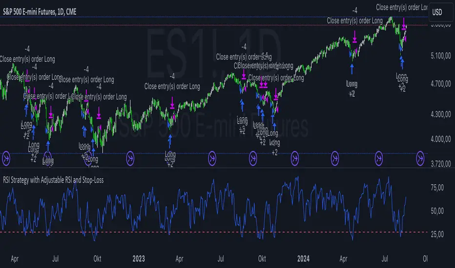
RSI Strategy with Adjustable RSI and Stop-LossThis trading strategy uses the Relative Strength Index (RSI) and a Stop-Loss mechanism to make trading decisions. Here’s a breakdown of how it works:
RSI Calculation:
The RSI is calculated based on the user-defined length (rsi_length). This is a momentum oscillator that measures the speed and change of price movements.
Buy Condition:
The strategy generates a buy signal when the RSI value is below a user-defined threshold (rsi_threshold). This condition indicates that the asset might be oversold and potentially due for a rebound.
Stop-Loss Mechanism:
Upon triggering a buy signal, the strategy calculates the Stop-Loss level. The Stop-Loss level is set to a percentage below the entry price, as specified by the user (stop_loss_percent). This level is used to limit potential losses if the price moves against the trade.
Sell Condition:
A sell signal is generated when the current closing price is higher than the highest high of the previous day. This condition suggests that the price has reached a new high, and the strategy decides to exit the trade.
Plotting:
The RSI values are plotted on the chart for visual reference. A horizontal line is drawn at the RSI threshold level to help visualize the oversold condition.
Summary
Buying Strategy: When RSI is below the specified threshold, indicating potential oversold conditions.
Stop-Loss: Set based on a percentage of the entry price to limit potential losses.
Selling Strategy: When the price surpasses the highest high of the previous day, signaling a potential exit point.
This strategy aims to capture potential rebounds from oversold conditions and manage risk using a Stop-Loss mechanism. As with any trading strategy, it’s essential to test and optimize it under various market conditions to ensure its effectiveness.
Double Bottom and Top Hunter### Türkçe Açıklama:
Bu strateji, grafikte ikili dip ve ikili tepe formasyonlarını tespit ederek otomatik alım ve satım işlemleri gerçekleştirir. İkili dip, fiyatın belirli bir dönem içinde iki kez en düşük seviyeye ulaşması ile oluşur ve bu durumda strateji long (alım) işlemi açar. İkili tepe ise fiyatın belirli bir dönem içinde iki kez en yüksek seviyeye ulaşması ile oluşur ve bu durumda strateji short (satış) işlemi açar.
- **Dönem Uzunluğu ve Geriye Dönük Kontrol:** Strateji, varsayılan olarak 100 periyotluk bir zaman dilimini temel alır ve bu süre boyunca en düşük ve en yüksek fiyat seviyelerini belirler. Geriye dönük kontrol süresi de 100 periyot olarak ayarlanmıştır.
- **İşlem Açma Koşulları:** İkili dip tespit edildiğinde long pozisyon, ikili tepe tespit edildiğinde short pozisyon açılır.
- **İşlem Kapatma Koşulları:** İkili dipte, en yüksek seviyeye (HH) ulaşıldıktan sonra fiyatın daha düşük bir seviye (LL) yapması durumunda pozisyon kapanır. İkili tepede ise tam tersi bir durumda, pozisyon kapanır.
- **Zigzag Çizimi:** İkili dip ve tepe formasyonları, grafik üzerinde yeşil (dipler) ve kırmızı (tepeler) zigzag çizgileri ile gösterilir.
Bu strateji, özellikle 1, 3 ve 5 dakikalık kısa zaman dilimlerinde yüksek başarı oranına sahiptir ve piyasadaki kısa vadeli trend dönüşlerini yakalamada etkili bir araçtır.
### English Explanation:
This strategy automatically executes buy and sell orders by detecting double bottom and double top formations on the chart. A double bottom occurs when the price reaches a low level twice within a specific period, prompting the strategy to open a long (buy) position. Conversely, a double top forms when the price reaches a high level twice, leading the strategy to open a short (sell) position.
- **Period Length and Lookback Control:** By default, the strategy is based on a 100-period length, during which it identifies the lowest and highest price levels. The lookback control period is also set to 100 periods.
- **Entry Conditions:** A long position is opened when a double bottom is detected, while a short position is opened when a double top is identified.
- **Exit Conditions:** In the case of a double bottom, the position is closed after the price reaches a higher high (HH) and then makes a lower low (LL). For a double top, the opposite occurs before closing the position.
- **Zigzag Plotting:** The double bottom and top formations are visually represented on the chart with green (bottoms) and red (tops) zigzag lines.
This strategy is particularly successful in short timeframes such as 1, 3, and 5 minutes and is an effective tool for capturing short-term trend reversals in the market.
Multi-Step FlexiSuperTrend - Strategy [presentTrading]At the heart of this endeavor is a passion for continuous improvement in the art of trading
█ Introduction and How it is Different
The "Multi-Step FlexiSuperTrend - Strategy " is an advanced trading strategy that integrates the well-known SuperTrend indicator with a nuanced and dynamic approach to market trend analysis. Unlike conventional SuperTrend strategies that rely on static thresholds and fixed parameters, this strategy introduces multi-step take profit mechanisms that allow traders to capitalize on varying market conditions in a more controlled and systematic manner.
What sets this strategy apart is its ability to dynamically adjust to market volatility through the use of an incremental factor applied to the SuperTrend calculation. This adjustment ensures that the strategy remains responsive to both minor and major market shifts, providing a more accurate signal for entries and exits. Additionally, the integration of multi-step take profit levels offers traders the flexibility to scale out of positions, locking in profits progressively as the market moves in their favor.
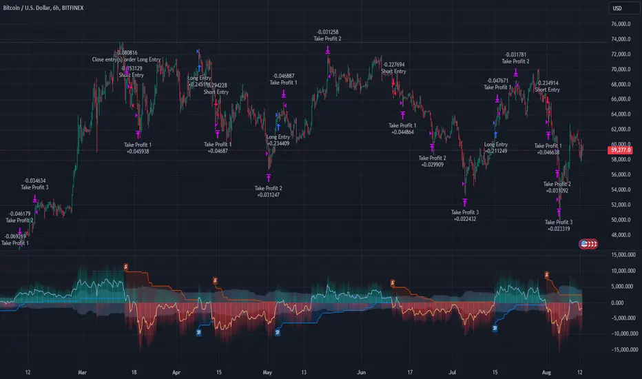
BTC 6hr Long/Short Performance
█ Strategy, How it Works: Detailed Explanation
The Multi-Step FlexiSuperTrend strategy operates on the foundation of the SuperTrend indicator, but with several enhancements that make it more adaptable to varying market conditions. The key components of this strategy include the SuperTrend Polyfactor Oscillator, a dynamic normalization process, and multi-step take profit levels.
🔶 SuperTrend Polyfactor Oscillator
The SuperTrend Polyfactor Oscillator is the heart of this strategy. It is calculated by applying a series of SuperTrend calculations with varying factors, starting from a defined "Starting Factor" and incrementing by a specified "Increment Factor." The indicator length and the chosen price source (e.g., HLC3, HL2) are inputs to the oscillator.
The SuperTrend formula typically calculates an upper and lower band based on the average true range (ATR) and a multiplier (the factor). These bands determine the trend direction. In the FlexiSuperTrend strategy, the oscillator is enhanced by iteratively applying the SuperTrend calculation across different factors. The iterative process allows the strategy to capture both minor and significant trend changes.
For each iteration (indexed by `i`), the following calculations are performed:
1. ATR Calculation: The Average True Range (ATR) is calculated over the specified `indicatorLength`:
ATR_i = ATR(indicatorLength)
2. Upper and Lower Bands Calculation: The upper and lower bands are calculated using the ATR and the current factor:
Upper Band_i = hl2 + (ATR_i * Factor_i)
Lower Band_i = hl2 - (ATR_i * Factor_i)
Here, `Factor_i` starts from `startingFactor` and is incremented by `incrementFactor` in each iteration.
3. Trend Determination: The trend is determined by comparing the indicator source with the upper and lower bands:
Trend_i = 1 (uptrend) if IndicatorSource > Upper Band_i
Trend_i = 0 (downtrend) if IndicatorSource < Lower Band_i
Otherwise, the trend remains unchanged from the previous value.
4. Output Calculation: The output of each iteration is determined based on the trend:
Output_i = Lower Band_i if Trend_i = 1
Output_i = Upper Band_i if Trend_i = 0
This process is repeated for each iteration (from 0 to 19), creating a series of outputs that reflect different levels of trend sensitivity.
Local
🔶 Normalization Process
To make the oscillator values comparable across different market conditions, the deviations between the indicator source and the SuperTrend outputs are normalized. The normalization method can be one of the following:
1. Max-Min Normalization: The deviations are normalized based on the range of the deviations:
Normalized Value_i = (Deviation_i - Min Deviation) / (Max Deviation - Min Deviation)
2. Absolute Sum Normalization: The deviations are normalized based on the sum of absolute deviations:
Normalized Value_i = Deviation_i / Sum of Absolute Deviations
This normalization ensures that the oscillator values are within a consistent range, facilitating more reliable trend analysis.
For more details:
🔶 Multi-Step Take Profit Mechanism
One of the unique features of this strategy is the multi-step take profit mechanism. This allows traders to lock in profits at multiple levels as the market moves in their favor. The strategy uses three take profit levels, each defined as a percentage increase (for long trades) or decrease (for short trades) from the entry price.
1. First Take Profit Level: Calculated as a percentage increase/decrease from the entry price:
TP_Level1 = Entry Price * (1 + tp_level1 / 100) for long trades
TP_Level1 = Entry Price * (1 - tp_level1 / 100) for short trades
The strategy exits a portion of the position (defined by `tp_percent1`) when this level is reached.
2. Second Take Profit Level: Similar to the first level, but with a higher percentage:
TP_Level2 = Entry Price * (1 + tp_level2 / 100) for long trades
TP_Level2 = Entry Price * (1 - tp_level2 / 100) for short trades
The strategy exits another portion of the position (`tp_percent2`) at this level.
3. Third Take Profit Level: The final take profit level:
TP_Level3 = Entry Price * (1 + tp_level3 / 100) for long trades
TP_Level3 = Entry Price * (1 - tp_level3 / 100) for short trades
The remaining portion of the position (`tp_percent3`) is exited at this level.
This multi-step approach provides a balance between securing profits and allowing the remaining position to benefit from continued favorable market movement.
█ Trade Direction
The strategy allows traders to specify the trade direction through the `tradeDirection` input. The options are:
1. Both: The strategy will take both long and short positions based on the entry signals.
2. Long: The strategy will only take long positions.
3. Short: The strategy will only take short positions.
This flexibility enables traders to tailor the strategy to their market outlook or current trend analysis.
█ Usage
To use the Multi-Step FlexiSuperTrend strategy, traders need to set the input parameters according to their trading style and market conditions. The strategy is designed for versatility, allowing for various market environments, including trending and ranging markets.
Traders can also adjust the multi-step take profit levels and percentages to match their risk management and profit-taking preferences. For example, in highly volatile markets, traders might set wider take profit levels with smaller percentages at each level to capture larger price movements.
The normalization method and the incremental factor can be fine-tuned to adjust the sensitivity of the SuperTrend Polyfactor Oscillator, making the strategy more responsive to minor market shifts or more focused on significant trends.
█ Default Settings
The default settings of the strategy are carefully chosen to provide a balanced approach between risk management and profit potential. Here is a breakdown of the default settings and their effects on performance:
1. Indicator Length (10): This parameter controls the lookback period for the ATR calculation. A shorter length makes the strategy more sensitive to recent price movements, potentially generating more signals. A longer length smooths out the ATR, reducing sensitivity but filtering out noise.
2. Starting Factor (0.618): This is the initial multiplier used in the SuperTrend calculation. A lower starting factor makes the SuperTrend bands closer to the price, generating more frequent trend changes. A higher starting factor places the bands further away, filtering out minor fluctuations.
3. Increment Factor (0.382): This parameter controls how much the factor increases with each iteration of the SuperTrend calculation. A smaller increment factor results in more gradual changes in sensitivity, while a larger increment factor creates a wider range of sensitivity across the iterations.
4. Normalization Method (None): The default is no normalization, meaning the raw deviations are used. Normalization methods like Max-Min or Absolute Sum can make the deviations more consistent across different market conditions, improving the reliability of the oscillator.
5. Take Profit Levels (2%, 8%, 18%): These levels define the thresholds for exiting portions of the position. Lower levels (e.g., 2%) capture smaller profits quickly, while higher levels (e.g., 18%) allow positions to run longer for more significant gains.
6. Take Profit Percentages (30%, 20%, 15%): These percentages determine how much of the position is exited at each take profit level. A higher percentage at the first level locks in more profit early, reducing exposure to market reversals. Lower percentages at higher levels allow for a portion of the position to benefit from extended trends.
Fine-tune Inputs: Gann + Laplace Smooth Volume Zone OscillatorUse this Strategy to Fine-tune inputs for the GannLSVZ0 Indicator.
Strategy allows you to fine-tune the indicator for 1 TimeFrame at a time; cross Timeframe Input fine-tuning is done manually after exporting the chart data.
I suggest using "Close all" input False when fine-tuning Inputs for 1 TimeFrame. When you export data to Excel/Numbers/GSheets I suggest using "Close all" input as True, except for the lowest TimeFrame.
MEANINGFUL DESCRIPTION:
The Volume Zone oscillator breaks up volume activity into positive and negative categories. It is positive when the current closing price is greater than the prior closing price and negative when it's lower than the prior closing price. The resulting curve plots through relative percentage levels that yield a series of buy and sell signals, depending on level and indicator direction.
The Gann Laplace Smoothed Volume Zone Oscillator GannLSVZO is a refined version of the Volume Zone Oscillator, enhanced by the implementation of the upgraded Discrete Fourier Transform, the Laplace Stieltjes Transform. Its primary function is to streamline price data and diminish market noise, thus offering a clearer and more precise reflection of price trends.
By combining the Laplace with Gann Swing Entries and with Ehler's white noise histogram, users gain a comprehensive perspective on volume-related market conditions.
HOW TO USE THE INDICATOR:
The default period is 2 but can be adjusted after backtesting. (I suggest 5 VZO length and NoiceR max length 8 as-well)
The VZO points to a positive trend when it is rising above the 0% level, and a negative trend when it is falling below the 0% level. 0% level can be adjusted in setting by adjusting VzoDifference. Oscillations rising below 0% level or falling above 0% level result in a natural trend.
HOW TO USE THE STRATEGY:
Here you fine-tune the inputs until you find a combination that works well on all Timeframes you will use when creating your Automated Trade Algorithmic Strategy. I suggest 4h, 12h, 1D, 2D, 3D, 4D, 5D, 6D, W and M.
When Indicator/Strategy returns 0 or natural trend, Strategy Closes All it's positions.
ORIGINALITY & USFULLNESS:
Personal combination of Gann swings and Laplace Stieltjes Transform of a price which results in less noise Volume Zone Oscillator.
The Laplace Stieltjes Transform is a mathematical technique that transforms discrete data from the time domain into its corresponding representation in the frequency domain. This process involves breaking down a signal into its individual frequency components, thereby exposing the amplitude and phase characteristics inherent in each frequency element.
This indicator utilizes the concept of Ehler's Universal Oscillator and displays a histogram, offering critical insights into the prevailing levels of market noise. The Ehler's Universal Oscillator is grounded in a statistical model that captures the erratic and unpredictable nature of market movements. Through the application of this principle, the histogram aids traders in pinpointing times when market volatility is either rising or subsiding.
The Gann swing strategy is developed by meomeo105, this Gann high and low algorithm forms the basis of the EMA modification.
DETAILED DESCRIPTION:
My detailed description of the indicator and use cases which I find very valuable.
What is oscillator?
Oscillators are chart indicators that can assist a trader in determining overbought or oversold conditions in ranging (non-trending) markets.
What is volume zone oscillator?
Price Zone Oscillator measures if the most recent closing price is above or below the preceding closing price.
Volume Zone Oscillator is Volume multiplied by the 1 or -1 depending on the difference of the preceding 2 close prices and smoothed with Exponential moving Average.
What does this mean?
If the VZO is above 0 and VZO is rising. We have a bullish trend. Most likely.
If the VZO is below 0 and VZO is falling. We have a bearish trend. Most likely.
Rising means that VZO on close is higher than the previous day.
Falling means that VZO on close is lower than the previous day.
What if VZO is falling above 0 line?
It means we have a high probability of a bearish trend.
Thus the indicator returns 0 and Strategy closes all it's positions when falling above 0 (or rising bellow 0) and we combine higher and lower timeframes to gauge the trend.
What is approximation and smoothing?
They are mathematical concepts for making a discrete set of numbers a
continuous curved line.
Laplace Stieltjes Transform approximation of a close price are taken from aprox library.
Key Features:
You can tailor the Indicator/Strategy to your preferences with adjustable parameters such as VZO length, noise reduction settings, and smoothing length.
Volume Zone Oscillator (VZO) shows market sentiment with the VZO, enhanced with Exponential Moving Average (EMA) smoothing for clearer trend identification.
Noise Reduction leverages Euler's White noise capabilities for effective noise reduction in the VZO, providing a cleaner and more accurate representation of market dynamics.
Choose between the traditional Fast Laplace Stieltjes Transform (FLT) and the innovative Double Discrete Fourier Transform (DTF32) soothed price series to suit your analytical needs.
Use dynamic calculation of Laplace coefficient or the static one. You may modify those inputs and Strategy entries with Gann swings.
I suggest using "Close all" input False when fine-tuning Inputs for 1 TimeFrame. When you export data to Excel/Numbers/GSheets I suggest using "Close all" input as True, except for the lowest TimeFrame. I suggest using 100% equity as your default quantity for fine-tune purposes. I have to mention that 100% equity may lead to unrealistic backtesting results. Be avare. When backtesting for trading purposes use Contracts or USDT.

Project Monday Strategy [AlgoAI System]Overview
Project Monday is a sophisticated trading strategy designed for active market participants. This strategy can be used alongside other forms of technical analysis, providing traders with additional tools to enhance their market insights. While it offers a flexible approach for identifying and exploiting market inefficiencies, Project Monday does not fit every market condition and requires adjustments. Its core principles include technical analysis and risk management, all aimed at making informed trading decisions and managing risk effectively.
Features
Project Monday Strategy works in any market and includes many features:
Efficient Trading Presets: Offers ready-to-use presets that allow traders to start efficient trading with one click.
Confirmation Signals: Provides signals to help traders validate trends, emphasizing informed decision-making (not to be followed blindly).
Reversal Signals: Identifies signals to alert traders to potential reversals, encouraging careful analysis (not to be followed blindly).
Adaptability: Can be adjusted to fit different market conditions, ensuring ongoing effectiveness.
Multi-Market Application: Suitable for use across various asset classes including stocks, forex, commodities, and cryptocurrencies.
Integration: Can be used alongside other technical analysis tools for enhanced decision-making.
Position Sizing: Allows traders to determine optimal trade size using backtesting and trading performance dashboard.
Backtesting: Supports historical testing to refine and validate the strategy.
Continuous Monitoring: Includes features for ongoing performance evaluation and strategy adjustments.
Unique Project Monday Strategy Features on TradingView:
Adaptive Position Sizing: Dynamically adjusts the size of each position based on market conditions and predefined risk management criteria, ensuring optimal trade sizing and risk exposure.
Preliminary Position Opening: Allows traders to enter a position in anticipation of a signal confirmation, enabling them to capture early market movements and improve entry points.
Preliminary Position Closing: Enables traders to exit a position before a signal reversal, helping to lock in profits and minimize potential losses during volatile market conditions.
Adjusting Strategy Parameters:
Price Band Inputs:
Project Monday Strategy uses a set of configurable inputs to tailor its behavior according to the trader's preferences. The following are the key inputs for the price band calculations. Signals are not generated when the price remains within these bands.
“Length of Calculation” determines how many historical data points are used in the trend calculation. A shorter “Length of Calculation” will make the Price Band more responsive to recent price changes but may also increase the noise and the likelihood of false signals. A longer “Length of Calculation” will make the Price Band smoother, with less noise, but may cause more lag in reacting to price changes.
“Offset” determines the position of the Gaussian filter, which is used to weight the data points in the trend calculation. The offset is expressed as a fraction of the “Length of Calculation”, with a value between 0 and 1. A higher “Offset” will shift the Gaussian filter closer to the more recent data points, making the Price Band more responsive to recent price changes but potentially increasing noise. A lower “Offset” will shift the Gaussian filter closer to the centre of the window, resulting in a smoother Price Band but potentially introducing more lag.
“Sigma” refers to the standard deviation used in the Gaussian distribution function. This parameter determines the smoothness of the curve and the degree to which data points close to the centre of the “Length of Calculation” are weighted more heavily than those further away. A smaller “Sigma” will result in a narrower Gaussian filter, leading to a more responsive Price Band but with a higher chance of noise and false signals. A larger “Sigma” will result in a wider Gaussian filter, creating a smoother Price Band but with more lag.
Adjust the “Source” inputs to specify which type of price data should be used for strategy calculations and signal generation.
“Width of Band” input determines the multiplier for the band width. A higher value of “Width of Band” makes the price band wider, which generates fewer signals due to the lower probability of the price moving outside the band. Conversely, a lower multiplier makes the band narrower, generating more signals but also increasing the likelihood of false signals.
Direction input:
The Project Monday strategy includes an input to specify the direction of trades, allowing traders to control whether the strategy should consider long positions, short positions, or both. The following input parameter is used for this purpose:
This input parameter allows traders to define the type of positions the strategy will take. It has three options:
Only Long: The strategy will generate signals exclusively for buying or closing short positions, focusing on potential uptrends.
Only Short: The strategy will generate signals exclusively for selling or closing long positions, focusing on potential downtrends.
Both: The strategy will generate signals for both buying (long positions) and selling (short positions), allowing for a more comprehensive trading approach that captures opportunities in both rising and falling markets.
Signals Filter:
The Project Monday strategy includes inputs to filter signals based on higher timeframes and the length of the data used for filtering. These inputs help traders refine the strategy's performance by considering broader market trends and smoothing out short-term fluctuations.
Filter Timeframe input specifies the timeframe used for filtering signals. By choosing a higher timeframe, traders can filter out noise from shorter timeframes and focus on more significant trends. The options range from intraday minutes (e.g., 1, 5, 15 minutes) to daily (1D, 2D, etc.), weekly (1W, 2W, etc.), and monthly (1M) timeframes. This allows traders to align their strategy with their preferred trading horizon and market perspective.
Filter Length input defines the number of data points used for filtering signals on the selected timeframe. A longer filter length will smooth out the data more, helping to identify sustained trends and reduce the impact of short-term fluctuations. Conversely, a shorter filter length will make the filter more responsive to recent price changes, potentially generating more signals but also increasing sensitivity to market noise.
Adaptive Position Size:
The Project Monday strategy incorporates inputs for unique feature Adaptive Position Sizing (APS), which dynamically adjusts the size of trades based on market conditions and specified parameters. This feature helps optimize risk management and trading performance.
Enable Adaptive Position Size: Users can check or uncheck this box to enable or disable the Adaptive Position Size feature. When checked, the strategy dynamically adjusts position sizes based on the defined parameters. This allows traders to scale their positions according to market volatility and other factors, enhancing risk management and potentially improving returns. When unchecked, the strategy will not adjust position sizes adaptively, and positions will remain fixed as per other settings.
“Timeframe for Adaptive Position Size “input specifies the timeframe used for calculating the position size. Options range from intraday minutes (e.g., 30, 60 minutes) to daily (1D, 3D), weekly (1W), and monthly (1M) timeframes. Selecting an appropriate timeframe helps align position sizing calculations with the trader’s overall strategy and market perspective, ensuring that position sizes are adjusted based on relevant market data.
“APS Length” input defines the number of data points used to calculate the adaptive position size. A longer APS length will result in higher position sizes. Conversely, a shorter APS length will result in smaller position sizes.
Anticipatory Trading:
Project Monday Strategy includes inputs for unique feature Anticipatory Trading, allowing traders to open and close positions preliminarily based on certain conditions. This feature aims to provide an edge by taking action before traditional signals confirm.
Enable Preliminary Position Opening: Users can check or uncheck this box to enable or disable Preliminary Position Opening. When enabled, the strategy will open positions based on preliminary conditions before the standard signals are confirmed. This can help traders capitalize on early trend movements and potentially gain a better entry point.
Enable Preliminary Position Closing: Users can check or uncheck this box to enable or disable Preliminary Position Closing. When enabled, the strategy will close positions based on preliminary conditions before the standard exit signals are confirmed. This can help traders lock in profits or limit losses by exiting positions at the early signs of trend reversals.
“Position Size in %” input specifies the position size as a percentage of the trading capital. By setting this value, traders can control the amount of capital allocated to each trade. For example, a risk value of 40% means that 40% of the available trading capital will be used for each anticipatory trade. This helps in managing risk and ensuring that the position size aligns with the trader's risk tolerance and overall strategy.
Usage:
Signal Generation
Long signal indicates a potential uptrend, suggesting either buying or closing a short position. Short signal indicates a potential downtrend, suggesting either selling or closing a long position. Signals are generated on your chart when the price moves beyond a calculated price band based on the current trend.
Signal Filtering
The strategy includes a filtering mechanism based on the current or another timeframe. Filtering works best with higher timeframes. This component calculates the trend on a higher timeframe and predicts the trend, ensuring trades on the current timeframe are only opened if they align with the higher timeframe trend. Setting the right filter timeframe is crucial for obtaining the best signals.
Position Direction
Users can choose the direction of positions to open via the settings box. Options include only long positions, only short positions, or both.
Adaptive Position Size (APS)
Users can enable the Adaptive Position Size feature to adjust position sizes based on trend strength. The strategy evaluates the strength of the current trend based on a higher timeframe. The stronger the trend, the larger the position size for opening a position.
Anticipatory Trading
Users can activate this unique feature to enhance trading decisions. The strategy assesses the likelihood of receiving a main signal. If the opportunity appears strong, it opens a partial position, as specified in the settings box. As the probability of the signal strengthens, the strategy gradually increases the position size.
Exit Strategy
The strategy exits positions based on receiving a reverse signal. Positions opened through “Anticipatory trading” are exited incrementally as each preliminary signal reverses.
By following these steps, traders can implement the strategy to navigate various market scenarios, manage risk, and adjust trading performance over time. Adjusting parameters and monitoring signals diligently are key to adapting the strategy to individual trading styles and market conditions.
You will get
By purchasing the Project Monday strategy, you not only gain access to a cutting-edge system but also receive ready-to-use presets designed to help you start trading immediately and achieve optimal results. Additionally, you benefit from comprehensive support and the option to request custom presets for your desired financial instruments through our dedicated support team, ensuring you have the tools and assistance needed for successful trading.
Risk Disclaimer
This information is not a personalized investment recommendation, and the financial instruments or transactions mentioned in it may not be appropriate for your financial situation, investment objective(s), risk tolerance, and/or expected return. AlgoAI shall not be liable for any losses incurred in the event of transactions or investments in financial instruments mentioned in this information.

Self Optimizing RSI and Self Adaptive TP/SL [Starbots]Self Optimizing RSI and Self Adaptive TP/SL Strategy. (non-repainting)
This script continuously backtests 20 different combinations of RSI Buy conditions across 5 different Take Profit/Stop Loss combinations. In total, it tests 100 variants on every bar close and records the Net Profit gained for each combination. The strategy then selects and uses the best-performing combination of settings currently available for you to trade.
---------------------------------------------------------------------------------------------------------
The Relative Strength Index (RSI), developed by J. Welles Wilder, is a momentum oscillator that measures the speed and change of price movements. The RSI oscillates between zero and 100. Traditionally the RSI is considered overbought when above 70 and oversold when below 30. Signals can be generated by looking for divergences and failure swings. RSI can also be used to identify the general trend.
To improve our results we are calculating Multiple Length RSI - Average RSI based on the multiple periods. You can use just 1 Length or Multiple.
Set Inputs to Min=14, Max=14 if you want to use just 1 period.
= RSI(14)
3 RSI Lengths example (12,13 and 14):
Min=12, Max=14
(12+13+14) / 3 = avg. RSI
-----------------------------------------------------------------------------------------------------------
Backtester - Optimizer Explained:
The backtester runs numerous backtests in the background to optimize trading strategies. Here’s how it works:
Default Inputs (Combinations of TP/SL)
TP 1%, SL4%
TP 2%, SL4%
TP 3%, SL4%
TP 2%, SL5%
TP 4.5%, SL10%
Default Inputs (RSI Crossover Buys) :
18 ,20,21,22,23,24,25,26,27,28,29,30,31,32,33,34,35,45,55, 69
_______________________________________________________
Backtest RSI Crossover 18:
TP1%, SL4% => Save net profit
TP2%, SL4% => Save net profit
TP3%, SL4% => Save net profit
TP2%, SL5% => Save net profit
TP4.5%, SL10% => Save net profit
,...
,...
Backtest RSI Crossover 69:
TP1%, SL4% => Save net profit
TP2%, SL4% => Save net profit
TP3%, SL4% => Save net profit
TP2%, SL5% => Save net profit
TP4.5%, SL10% => Save net profit
Self Optimizing Buy Condition and Self Optimizing Take Profit - Stop Los
This process involves testing various combinations of RSI crossover values with different Take Profit (TP) and Stop Loss (SL) percentages. The net profit for each combination is saved, allowing the optimizer to select the best-performing settings for trading.
It recalculates on every bar close. If one combination starts performing better than others—achieving a higher net profit gain (essentially like running 100 backtests with different settings in the background)—the strategy switches to that combination of TP/SL and Buy condition. It continues trading with the new settings until another parameter starts performing better and the strategy switches to that setting.
________________________________________________________________________
If you wish to use it as INDICATOR - turn on 'Recalculate - On every tick' in Properties tab to have this script updating constantly and use it as a normal Indicator tool for manual trading.
Other functions:
Set the %fee for optimizing engine. If you set this % higher, you also punish small average trades and make the strategy prefer larger avg. trades, giving you better chances to make your strategy profitable.
Trade with trend and optimize the strategy only when the market is uptrending with EMA/HMA
Use Moving Average of avg.RSI and smooth the values for indicator even more. (Yes strategy is self optimizing RSI or avg.RSI or RSI-MA, you can select all sorts of this indicator for optimizing)
All trading alerts are working and functional, if you want to automate the strategy
This script is simple to use for any trader as it saves a lot of time for searching good parameters on your own. It's self-optimizing and adjusting to the markets on the go.

Moving Average Crossover Swing StrategyMoving Average Crossover Swing Strategy
**Overview:**
The basic concept of this strategy is to generate a signal when a faster/shorter length moving average crosses over (for Longs) or crosses under (for Shorts) a medium/longer length moving average. All of which are customizable. This strategy can work on any timeframe, however the daily is the timeframe used for the default settings and screenshots, as it was designed to be a multi-day swing strategy. Once a signal has been confirmed with a candle close, based on user options, the strategy will enter the trade on the open of the next candle.
The crossover strategy is nothing new to trading, but what can make this strategy unique and helpful, is the addition of further confirmation points, ATR based stop loss and take profit targets, optional early exit criteria, customizable to your needs and style, and just about everything visual can be toggled on/off. This strategy is based on a Trend (MA) indicator and a Momentum (MACD) indicator. While a Volume-based indicator is not shown here, one could consider using their favorite from that category to further compliment the signal idea.
It should be noted that depending on the time frame, direction(s) chosen, the signal options, confirmation options, and exit options selected, that a ticker may not produce more than 100 trades on the back test. Depending on your style and frequency, one could consider adjusting options and/or testing multiple tickers. It should also be noted that this strategy simply tests the underlying stock prices, not options contracts. And of course, testing this strategy against historical data does not assume that the same results will occur in future price action.
Shoutout given to Ripster's Clouds Indicator as pieces of that code were taken and modified to create both the Cloud visualization effects, and the Moving Average Pair Plots that are implemented in this strategy.
BASIC DEFAULTS
All can be changed as normal
Initial capital = 10,000
Order Sizing = 25% of equity (use the "Inputs" tab to modify this)
Pyramiding = 0
Commission = 0.65 USD per order
Price Verification = 1 tick
Slippage = 1 tick
RISK MANAGMENT
You will notice two different percentage options and ATR multipliers. This strategy will adjust position sizing by not exceeding either one of those % values based on the ATR (Average True Range) of the symbol and the multipliers selected, should the stock hit the stop loss price.
For Example, lets assume these values are true:
Account size = $10,000,
Max Risk = 1% of account size
Max Position Size = 25% of the account size
Stock Price = 23.45
ATR = 3.5
ATR Stop Loss Multiplier = 1.4
Then the formulas would be:
ACCT_SIZE * MaxRisk_% = 10000 * .01 = $100 (MaxCashRisk)
-----
MaxCashRisk / (ATR * ATR_SL_MULTIPLIER) = 100 / (3.5 * 1.4) = 20.4 Shares based on Max Cash Risk
-----
(ACCT_SIZE * MaxEquity_%) / STOCK_PRICE = (10000 * .25) / 23.45 = 106.61 Shares based on Max Equity Allocation
The minimum value of each of those options is then used, which in this case would be to purchase 20 shares so as not to exceed the max dollar risk should the stock reach the stop loss target. Likewise, if the ATR were to be much lower, say 0.48 cents, and all else the same, then the strategy would purchase the 106 shares based on Max Equity Allocation because the Max Cash Risk would require 149.25 shares.
MOVING AVERAGE OPTIONS
Select between and change the length & type of up to 5 pairs (10 total) of moving averages
The "Show Cloud-x" option will display a fill color between the "a" and "b" pairs
All moving averages lines can be toggled on/off in the "Style" tab, as well as adjusting their colors.
Visualization features do not affect calculations, meaning you could have all or nothing on the chart and the strategy will still produce results
SIGNAL CHOICES
Choose the fast/shorter length MA and the medium/longer length MA to determine the entry signal
CONFIRMATION OPTIONS
Both of these have customizable values and can be toggled on/off
A candle close over a slower/much longer length moving average
An additional cross-over (cross-under for Shorts) on the MACD indicator using default MACD values. While the MACD indicator is not necessary to have on the chart, it can help to add that for visualization. The calculations will perform whether the indicator is on the chart or not.
EARLY EXIT CRITERIA
Both can be toggled on/off with customizable values
MA Cross Exit will exit the trade early if the select moving averages cross-under (for longs) or cross-over (for shorts), indicating a potential reversal.
Max Bars in Trades will act as a last-resort exit by simply calculating the amount of full bars the trade has been open, and exiting on the opening of the next bar. For example: the default value is 8 bars, so after 8 full bars in the trade, if no other exit has been triggered (Stop Loss, Take Profit, or MA Cross(if enabled)), then the trade will exit at the opening of the 9th bar.
Finally, there is a table displaying the amount of trades taken for each side, and the amount & percent of both early exits. This table can be turned off in the "Style" tab
ADDITIONAL PLOTS
MACD (Moving Average Convergence/Divergence):
- The MACD is an optional confirmation indicator for this strategy.
- Plotting the indicator is not necessary for the strategy to work, but it can be helpful to visually see the status and position of the MACD if this feature is enabled in the strategy
- This helps to identify if there is also momentum behind the entry signal

TSI w SuperTrend decision - Strategy [presentTrading]This strategy aims to improve upon the performance of Traidngview's newly published "Trend Strength Index" indicator by incorporating the SuperTrend for better trade execution and risk management. Enjoy :)
█ Introduction and How it is Different
The "TSI with SuperTrend Decision - Strategy" combines the Trend Strength Index (TSI) with SuperTrend indicators to determine entry and exit points. Unlike traditional strategies that rely solely on one indicator, this method leverages the strengths of both TSI and SuperTrend to provide a more nuanced and adaptive trading strategy.
This dual approach allows for capturing trends more effectively, especially in volatile markets.
BTCUSD 8h LS Performance
█ Strategy, How it Works: Detailed Explanation
🔶 Trend Strength Index (TSI)
The TSI is a momentum oscillator that shows both the direction and strength of a trend. It is calculated by comparing the price movement with the bar index over a specified period. The formula for TSI is as follows:
```
TSI = (PC / |PC|)
where:
PC = Change in price over the period
```
In this strategy, TSI is calculated using the closing prices and a default period of 64 bars. The TSI values help identify overbought and oversold conditions, providing signals for potential market reversals.
🔶 SuperTrend Indicator
The SuperTrend is a trend-following indicator based on the average true range (ATR). It helps in identifying the direction of the market trend. The SuperTrend calculation involves:
```
SuperTrend = HLC3 ± (Factor * ATR)
where:
HLC3 = (High + Low + Close) / 3
Factor = User-defined multiplier
ATR = Average True Range over a period
```
The SuperTrend settings in this strategy include a length of 10 bars and a factor of 3.0.
Last Bull Cycle of BTC
🔶 Entry and Exit Conditions
The strategy uses the TSI and SuperTrend together to determine entry and exit points:
- Long Entry: When the SuperTrend indicates a downward trend (st.d < 0) and the TSI is above the oversold level (-0.241).
- Long Exit: When the SuperTrend indicates an upward trend (st.d > 0) and the TSI is below the overbought level (0.241).
- Short Entry: When the SuperTrend indicates an upward trend (st.d > 0) and the TSI is below the overbought level (0.241).
- Short Exit: When the SuperTrend indicates a downward trend (st.d < 0) and the TSI is above the oversold level (-0.241).
█ Trade Direction
The strategy allows users to select the trade direction through the `tradeDirection` input. The options are:
- Both: Enables both long and short trades.
- Long: Enables only long trades.
- Short: Enables only short trades.
█ Default Settings
- TSI Length: 64
- SuperTrend Length: 10
- SuperTrend Factor: 3.0
- Trade Direction: Both
- Take Profit (%): 30.0
- Stop Loss (%): 20.0
Impact of Default Settings
- TSI Length: A longer TSI period smooths out noise but may lag in identifying trends. A shorter period is more responsive but can generate false signals.
- SuperTrend Length: A shorter length provides quicker signals but can be prone to whipsaws. A longer length is more reliable but may delay entries and exits.
- SuperTrend Factor: A higher factor increases the distance of the SuperTrend from the price, reducing sensitivity to minor price fluctuations.
- Trade Direction: Allows flexibility in trading strategies by enabling both long and short trades based on market conditions.
- Take Profit and Stop Loss: These settings manage risk by automatically closing trades at predefined profit or loss levels. Higher percentages provide larger potential gains but also higher risk.

Universal Algo [Coff3eG]Universal Algo By G
Overview:
Universal Algo By G is a comprehensive LONG-ONLY trading strategy specifically designed for medium to long-term use in cryptocurrency markets, particularly Bitcoin. This algorithm can be manually adjusted to fit the volatility of specific coins, ensuring the best possible results. While it does not generate a large number of trades due to the nature of bull and bear market cycles, it has been rigorously backtested and forward-tested to ensure the strategy is not overfitted.
Core Features:
Integrated Systems: Universal Algo is built around five core systems, each contributing unique analytical perspectives to enhance trade signal reliability. These systems are designed to identify clear trend opportunities for significant gains while also employing logic to navigate through ranging markets effectively.
Optional Ranging Market Filter: Helps filter out noise, potentially enhancing signal clarity.
Market State Detection: Identifies four distinct market states:
Trending
Ranging
Danger (Possible top)
Possible Bottom
Global Liquidity Indicator (GLI) Integration: Leverages GLI values to identify positive liquidity trends.
Volatility Bands: Provides insights into market volatility.
Top and Bottom Detection: Shows possible bottoms with green backgrounds and red backgrounds for possible top detection.
The Market State Detection, GLI, Volatility Bands, and Top and Bottom Detection feature all serve as an expectation management feature.
Additional Features:
Optional Metrics Table: Displays strategy metrics and statistics, providing detailed insights into performance.
Customization Options: The script offers a range of user inputs, allowing for customization of the backtesting starting date, the decision to display the strategy equity curve, among other settings. These inputs cater to diverse trading needs and preferences, offering users control over their strategy implementation.
Operational Parameters:
Customizable Inputs: Users can adjust thresholds to match the coin's volatility, enhancing strategy performance.
Transparency and Logic Insight: While specific calculation details and proprietary indicators are integral to maintaining the uniqueness of Universal Algo, the strategy is grounded on well-established financial analysis techniques. These include momentum analysis, volatility assessments, and adaptive thresholding, among others, to formulate its trade signals. Notably, no single indicator is used in isolation; each indicator is combined with another to enhance signal accuracy and robustness. Some of the indicators include customized versions of the TEMA, Supertrend, Augmented Dickey-Fuller (ADF), and Weekly Positive Directional Movement Index (WPDM), all integrated together to create a cohesive and effective trading strategy.
System Operation:
Universal Algo works by taking the average score of the five core systems used for the signals. Three of these systems have been lengthened out to function as longer-term systems, while the remaining two operate at a slightly faster speed. This combination and averaging of systems help to balance the overall strategy, ensuring it maintains the right amount of speed to remain effective for medium to long-term use with minimal noise. The average score is then compared against customizable thresholds. The strategy will go long if the average score is above the threshold and short if it is below the threshold. This averaging mechanism helps to smooth out individual system anomalies and provides a more robust signal for trading decisions.
Originality and Usefulness:
Universal Algo is an original strategy that combines multiple proprietary and customized indicators to deliver robust trading signals. The strategy integrates various advanced indicators and methodologies, including:
System Indicator: Calculates a cumulative score based on recent price movements, aiding in trend detection.
Median For Loop: Utilizes percentile rank calculations of price data to gauge market direction.
Volatility Stop: A modified volatility-based stop-loss indicator that adjusts based on market conditions.
Supertrend: A customized supertrend indicator that uses percentile ranks and ATR for trend detection.
RSI and DEMA: Combines a modified RSI and DEMA for overbought/oversold conditions.
TEMA: Uses 3 different types of MA for trend detection and standard deviation bands for additional confirmation.
Detailed Explanation of Components and Their Interaction:
RSI (Relative Strength Index): Used to identify overbought and oversold conditions. In Universal Algo, RSI is combined with DEMA (Double Exponential Moving Average) to smooth the price data and provide clearer signals.
ATR (Average True Range): Used to measure market volatility. ATR is incorporated into the Volatility Stop and Supertrend indicators to adjust stop-loss levels and trend detection based on current market conditions.
DEMA (Double Exponential Moving Average): Provides a smoother price trend compared to traditional moving averages, reducing lag and making it easier to identify trend changes.
Modified TEMA (Triple Exponential Moving Average): Similar to DEMA but provides even greater smoothing, reducing lag further and enhancing trend detection accuracy.
Volatility Stop: Utilizes ATR to dynamically set stop-loss levels that adapt to changing market volatility. This helps in protecting profits and minimizing losses.
Customized Supertrend: Uses ATR and percentile ranks to determine trend direction and strength. This indicator helps in capturing major trends while filtering out market noise.
Median For Loop: Calculates percentile ranks of price data over a specified period to assess market direction. This helps in identifying potential reversals and trend continuations.
HMA (Hull Moving Average): A fast-acting moving average that reduces lag while maintaining smoothness. It helps in quickly identifying trend changes.
SMA (Simple Moving Average): A traditional moving average that provides baseline trend information. Combined with HMA and other indicators, it forms a comprehensive trend detection system.
Universal Algo offers a sophisticated blend of advanced indicators and proprietary logic that is not available in free or open-source scripts. Here are some reasons why it is worth paying for:
Customization and Flexibility: The strategy provides a high degree of customization, allowing users to adjust various parameters to suit their trading style and market conditions. This flexibility is often not available in free scripts.
Proprietary Indicators: The use of proprietary and customized indicators such as the TEMA, Supertrend, ADF, and WPDM ensures that the strategy is unique and not replicable by free or open-source scripts.
Integrated Systems: The strategy combines multiple systems and indicators to provide a more comprehensive and reliable trading signal. This integration helps to smooth out anomalies and reduces noise, providing clearer trading opportunities.
Rigorous Testing: Universal Algo has undergone extensive backtesting and forward-testing to ensure its robustness and reliability. The results demonstrate its ability to perform well under various market conditions, offering users confidence in its effectiveness.
Detailed Metrics and Analysis: The optional metrics table provides users with detailed insights into the strategy's performance, including metrics like equity, drawdown, Sharpe ratio, and more. This level of detail helps traders make informed decisions.
Value Addition: By providing a strategy that combines advanced indicators, customization options, and thorough testing, Universal Algo adds significant value to traders looking for a reliable and adaptable trading tool.
Realistic Trading Conditions:
Backtesting and Forward-Testing: Rigorous testing ensures performance and reliability, with a focus on prudent risk management. Default properties include an initial capital of $1000, 0 pyramiding, 20 slippage, 0.05% commission, and using 5% of equity for trades.
The strategy is designed and tested with a focus on achieving a balance between risk and reward, striving for robustness and reliability rather than unrealistic profitability promises. Realistic trading conditions are considered, including appropriate account size, commission, slippage, and sustainable risk levels per trade.
Concluding Thoughts:
Universal Algo By G is offered to the TradingView community as a robust tool for enhancing market analysis and trading strategies. It is designed with a commitment to quality, innovation, and adaptability, aiming to provide valuable insights and decision support across various market conditions. Potential users are encouraged to evaluate Universal Algo within the context of their overall trading approach and objectives.

Multi-Timeframe Trend Following with 200 EMA Filter - Longs OnlyOverview
This strategy is designed to trade long positions based on multiple timeframe Exponential Moving Averages (EMAs) and a 200 EMA filter. The strategy ensures that trades are only entered in strong uptrends and aims to capitalize on sustained upward movements while minimizing risk with a defined stop-loss and take-profit mechanism.
Key Components
Initial Capital and Position Sizing
Initial Capital: $1000.
Lot Size: 1 unit per trade.
Inputs
Fast EMA Length (fast_length): The period for the fast EMA.
Slow EMA Length (slow_length): The period for the slow EMA.
200 EMA Length (filter_length_200): Set to 200 periods for the primary trend filter.
Stop Loss Percentage (stop_loss_perc): Set to 1% of the entry price.
Take Profit Percentage (take_profit_perc): Set to 3% of the entry price.
Timeframes and EMAs
EMAs are calculated for the following timeframes using the request.security function:
5-minute: Short-term trend detection.
15-minute: Intermediate-term trend detection.
30-minute: Long-term trend detection.
The strategy also calculates a 200-period EMA on the 5-minute timeframe to serve as a primary trend filter.
Trend Calculation
The strategy determines the trend for each timeframe by comparing the fast and slow EMAs:
If the fast EMA is above the slow EMA, the trend is considered positive (1).
If the fast EMA is below the slow EMA, the trend is considered negative (-1).
Combined Trend Signal
The combined trend signal is derived by summing the individual trends from the 5-minute, 15-minute, and 30-minute timeframes.
A combined trend value of 3 indicates a strong uptrend across all timeframes.
Any combined trend value less than 3 indicates a weakening or negative trend.
Entry and Exit Conditions
Entry Condition:
A long position is entered if:
The combined trend signal is 3 (indicating a strong uptrend across all timeframes).
The current close price is above the 200 EMA on the 5-minute timeframe.
Exit Condition:
The long position is exited if:
The combined trend signal is less than 3 (indicating a weakening trend).
The current close price falls below the 200 EMA on the 5-minute timeframe.
Stop Loss and Take Profit
Stop Loss: Set at 1% below the entry price.
Take Profit: Set at 3% above the entry price.
These levels are automatically set when entering a trade using the strategy.entry function with stop and limit parameters.
Plotting
The strategy plots the fast and slow EMAs for the 5-minute timeframe and the 200 EMA for visual reference on the chart:
Fast EMA (5-min): Plotted in blue.
Slow EMA (5-min): Plotted in red.
200 EMA (5-min): Plotted in green.
Price-Volume Dynamic - Strategy [presentTrading]█ Introduction and How it is Different
The "Price-Volume Dynamic - Strategy" leverages a unique blend of price action, volume analysis, and statistical z-scores to establish trading positions. This approach differentiates itself by integrating the concept of the Point of Control (POC) from volume profile analysis with price-based z-score indicators to create a dynamic trading strategy. It tailors entry and exit thresholds based on current market volatility, providing a responsive and adaptive trading method. This strategy stands out by considering both historical volatility and price trends to adjust trading decisions in real-time, enhancing its effectiveness in various market conditions.
BTCUSD 4h LS Performance
█ Strategy: How It Works – Detailed Explanation
🔶 Calculating Point of Control (POC)
The Point of Control (POC) represents the price level with the highest traded volume over a specified lookback period. It's calculated by dividing the price range into a number of rows, each representing a price level. The volume at each price level is tallied and the level with the maximum volume is designated as the POC.
🔶 Dynamic Thresholds Adjustments
The entry and exit thresholds are dynamically adjusted based on normalized volatility, which is derived from the current, minimum, and maximum ATR over a specified period. This normalization ensures that the thresholds adapt to changes in market conditions, making the strategy sensitive to shifts in market volatility.
BTCUSD local performance
█ Trade Direction
The strategy can be configured to trade in three different directions: Long, Short, or Both. This flexibility allows traders to align their trading strategy with their market outlook or risk preferences. By adjusting the `POC_tradeDirection` input, traders can selectively participate in market movements that match their trading style and objectives.
█ Usage
To deploy this strategy, traders should apply it within a trading software that supports scripting and backtesting, such as TradingView's Pine Script environment. Users can input their parameters based on their analysis of the market conditions and their risk tolerance. It is essential for traders to backtest the strategy using historical data to evaluate its performance and make necessary adjustments before applying it in live trading scenarios.
█ Default Settings
- Lookback Length: Sets the period over which the highest and lowest prices, and the volume per price level, are calculated. A higher lookback length smoothens the volatility but may delay response to recent market movements.
- Number of Rows: Determines the granularity of price levels within the price range. More rows provide a more detailed volume profile but require more computational resources.
- Entry Z-Score Threshold Base: Influences the sensitivity of the strategy to enter trades. Higher values make the strategy more conservative, requiring stronger deviation from the mean to trigger a trade.
- Exit Z-Score Threshold Base: Sets the threshold for exiting trades, with lower values allowing trades to close on smaller price retractions, thereby potentially preserving profits or reducing losses.
- Trading Direction: Allows selection between Long, Short, or Both, enabling traders to tailor the strategy to their market view or risk preferences.
Trailing Take Profit - Close Based📝 Description
This script demonstrates a new approach to the trailing take profit.
Trailing Take Profit is a price-following technique. When used, instead of setting a limit order for the take profit target exiting from your position at the specified price, a stop order is conditionally set when the take profit target is reached. Then, the stop price (a.k.a trailing price), is placed below the take profit target at a distance defined by the user percentagewise. On regular time intervals, the stop price gets updated by following the "Trail Barrier" price (high by default) upwards. When the current price hits the stop price you exit the trade. Check the chart for more details.
This script demonstrates how to implement the close-based Trailing Take Profit logic for long positions, but it can also be applied for short positions if the logic is "reversed".
📢 NOTE
To generate some entries and showcase the "Trailing Take Profit" technique, this script uses the crossing of two moving averages. Please keep in mind that you should not relate the Backtesting results you see in the "Strategy Tester" tab with the success of the technique itself.
This is not a complete strategy per se, and the backtest results are affected by many parameters that are outside of the scope of this publication. If you choose to use this new approach of the "Trailing Take Profit" in your logic you have to make sure that you are backtesting the whole strategy.
⚔️ Comparison
In contrast to my older "Trailing Take Profit" publication where the trailing take profit implementation was tick-based, this new approach is close-based, meaning that the update of the stop price occurs at the bar close instead of every tick.
While comparing the real-time results of the two implementations is like comparing apples to oranges, because they have different dynamic behavior, the new approach offers better consistency between the backtesting results and the real-time results.
By updating the stop price on every bar close, you do not rely on the backtester assumptions anymore (check the Reasoning section below for more info).
The new approach resembles the conditional "Trailing Exit" technique, where the condition is true when the current price crosses over the take profit target. Then, the stop order is placed at the trailing price and it gets updated on every bar close to "follow" the barrier price (high). On the other hand, the older tick-based approach had more "tight" dynamics since the trailing price gets updated on every tick leaving less room for price fluctuations by making it more probable to reach the trailing price.
🤔 Reasoning
This new close-based approach addresses several practical issues the older tick-based approach had. Those issues arise mainly from the technicalities of the TV Backtester. More specifically, due to the assumptions the Broker Emulator makes for the price action of the history bars, the backtesting results in the TV Backtester are exaggerated, and depending on the timeframe, the backtesting results look way better than they are in reality.
The effect above, and the inability to reason about the performance of a strategy separated people into two groups. Those who never use this feature, because they couldn't know for sure the actual effect it might have in their strategy, (even if it turned out to be more profitable) and those who abused this type of "repainting" behavior to show off, and hijack some boosts from the community by boasting about the "fake" results of their strategies.
Even if there are ways to evaluate the effectiveness of the tick-based approach that is applied in an existing strategy (this is out of the topic of this publication), it requires extra effort to do the analysis. Using this closed-based approach we can have more predictable results, without surprises.
⚠️ Caveats
Since this approach updates the trailing price on bar close, you must wait for at least one bar to close after the price crosses over the take profit target.